Introduction to statistics
Many of the statistical tests detailed in subsequent pages of this module rely on the assumption that any continuous data approximates a normal distribution, or that the sample size is large enough that the sampling distribution of the mean approximates a normal distribution. But what exactly are the normal and sampling distributions, how large is a large enough sample and how do you know if a continuous variable is normally distributed? This page will address these questions, and is an important precursor to the content on inferential statistics covered in the following pages.
In brief, it covers the following:
- The definition of the normal distribution
- The definition of the sampling distribution
- How to test for normality
- Options for transforming variables if they are not normally distributed
The normal distribution
The normal distribution is a special kind of distribution that large amounts of naturally occurring continuous data (and hence also smaller samples of such data) often approximates. As a result, properties of the normal distribution are the underlying basis of calculations for many inferential statistical tests, called parametric tests. These key properties are as follows:
- The mean, median and mode are all equal in a normal distribution.
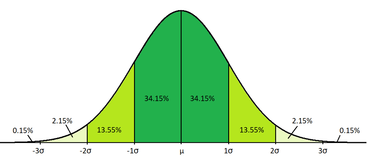
- Fixed proportions of the data lie within certain numbers of standard deviations from the mean in a normal distribution. In particular, 68% of the data lies within one standard deviation, 95% lies within two standard deviations and 99.7% lies within three standard deviations.
Given these properties, the graph of a normally distributed variable has a bell shape as shown below. Note that the percentages displayed here are given to two decimal places, while the percentages above are rounded values. Also note that the \(\mu\) and \(\sigma\) symbols represent population mean and population standard deviation respectively:
If you would like to practise interpreting a normally distributed data set, have a go at the following activity.
The sampling distribution
The descriptive statistics covered in the previous page of this module are used to analyse the data you have access to, which in most cases is a random sample of a larger population. It is important to note that a particular random sample from a population is only one of a number of possible samples though, and that values for sample statistics (e.g. the sample mean) can, in theory, be calculated for each possible sample of the same size. For example, we could measure the heights of a random sample of 100 Curtin students and obtain a mean of that sample, then we could do the same for a different random sample of 100 Curtin students, and for another sample, and so on and so on to calculate means for each possible sample of the same size.
All of these sample statistics (e.g. all of the means for our height example) have a distribution of their own, which is known as the sampling distribution. We could visualise this distribution using a histogram (as per any other data) if we had access to all the data, but note you wouldn’t usually do this as it would defeat the purpose of obtaining a random sample! Instead, inferential statistics estimate properties of the sampling distribution using data obtained from one random sample. The sampling distribution is therefore an important concept to be familiar with, and in particular it is important to be aware of these key properties of the sampling distribution of the mean:
- As the sample size increases, the shape of the sampling distribution of the mean becomes increasingly similar to the normal distribution. This is a very important theorem in statistics, and is called the Central Limit Theorem. Generally a sample size of 30 or more is considered large enough for the sampling distribution to approximate a normal distribution (although if the variable’s distribution is very skewed, a larger sample size may be required), and for this reason a sample size of 30 or more is usually enough to fulfil any normality requirements.
- The mean of the sampling distribution equals the mean of the population.
- The standard deviation of the sampling distribution equals the standard deviation of the population divided by the square root of the sample size. This is the standard error of the mean.
Testing for normality
If the inferential statistical test you wish to conduct requires a normally distributed continuous variable (or variables) and your sample size is not sufficiently large (typically 30 or above), then you will need to test to determine whether or not this is the case. Unfortunately there is not a single yes-or-no test for normality, and rather it requires assessing up to eight different factors in order to determine if the data approximates the normal distribution ‘closely enough’ (the data will never be perfectly normally distributed, and often a fair bit of deviation is acceptable). While some of these tests are more commonly used than others it is a good idea to evaluate as many as possible, particularly when you are first getting started, as the more information you have means the more complete of a picture you will have of your data, and the more well-informed your conclusion will be.
The eight statistics and graphs you can interpret are as follows:
-
Mean, median and mode
For a perfect normal distribution these three values should all be the same, so checking whether they are similar is a good (and simple) way to start. Note however that even in normally distributed data the mode may sometimes be higher or lower, but this is less of a concern than any differences between the mean and median. -
Skewness
Skewness measures the symmetry of the distribution. A skewness of \(0\) indicates a perfectly symmetrical distribution, while a negative value indicates negative skew (long tail to the left) and a positive value indicates positive skew (long tail to the right). If the data approximates a normal distribution the skewness should be close to \(0\), but a value within the range of \(-1\) to \(1\) is considered acceptable. Additionally, the z-score for the skewness, which can be calculated by dividing the skewness by its standard error, should be within the range of \(-1.96\) to \(1.96\) -
Kurtosis
Kurtosis measures the heaviness of the distribution’s tails. The kurtosis for the normal distribution is \(3\), although many researchers and software programs (e.g. SPSS) actually provide the excess kurtosis instead. This is calculated by subtracting \(3\) from the kurtosis, giving the normal distribution a value of \(0\). Using this measure, a positive kurtosis indicates wider tails and a negative kurtosis indicates narrower tails, but again a value within the range of \(−1\) to \(1\) is considered acceptable. Additionally, the z-score for the (excess) kurtosis, which can be calculated by dividing the (excess) kurtosis by its standard error, should be within the range of \(-1.96\) to \(1.96\) -
Normality test (e.g. Shapiro-Wilk)
The Shapiro-Wilk test is a normality test, which tests the null hypothesis that the distribution approximates a normal distribution (another normality test is the Kolmogorov-Smirnov test). A significance (\(p\)) value greater than \(0.05\) indicates that this null hypothesis should not be rejected, and therefore provides evidence that a normal distribution can be assumed (more on hypothesis testing is covered in the Inferential statistics page of this module). Note that this test is generally only used for sample sizes less than \(100\), as it can be too sensitive for larger samples. -
Histogram
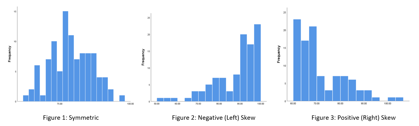
If the data is normally distributed the histogram should be approximately symmetric and centred around the mean (Figure 1). Alternatively, if there is a long tail to the left only it is skewed to the left (negatively skewed) (Figure 2), or if there is a long tail to the right only it is skewed to the right (positively skewed) (Figure 3):
-
Stem and leaf plot
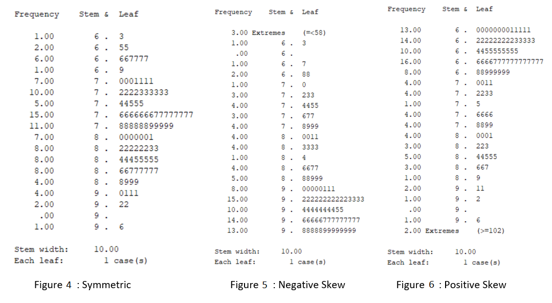
A stem and leaf plot displays the frequency of each value in the data set, organised into ‘stems’ and ‘leaves’. For example, Figure 4 below shows that there is one value of \(63\), two values of \(65\), six values of either \(66\) or \(67\), etc. This plot can be interpreted in the same way as a histogram, only rotated on its side.
-
Normal Q-Q plot
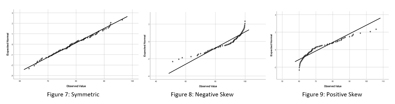
If the data is normally distributed the points on a normal Q-Q plot will fall approximately on the straight diagonal line (Figure 7). Otherwise, the points will not lie on the straight diagonal line (Figures 8 and 9). Note that another version of this plot, the detrended Q-Q plot, is sometimes also analysed. In the detrended plot there should be roughly equal number of points above and below the line, with no obvious trend.
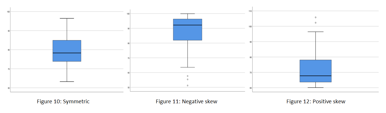
- Boxplot
If the data is normally distributed the median should be positioned approximately in the centre of the box, both whiskers should have similar length and ideally there should be no outliers (Figure 10). Alternatively, the boxplot may display a negative skew (Figure 11) or a positive skew (Figure 12):
After analysing the data relating to these tests of normality, you should come to an overall conclusion based on what the majority of the tests indicate. For example, your conclusion might be that the data is approximately normally distributed, or it might be that it is positively or negatively skewed.
For a worked example of assessing normality, you make like to view the Introduction to SPSS module. You can also practise assessing whether or not data approximates a normal distribution by having a go at the following activity.
Transforming variables
If tests for normality indicate that the variable is not normally distributed (and your sample size is not sufficiently large), you can try transforming the variable to see if it conforms more to the normal distribution. For example, if the data is negatively skewed you could try taking the square of the data, or if it is positively skewed you could try taking the natural logarithm (\(ln\)), the square root or the reciprocal.
Once the data has been transformed, it should be tested again for normality. If the transformation has ‘worked’, any further inferential analysis should be conducted on the transformed data. If it hasn’t, you will need to use non-parametric tests instead.