Introduction to Stata

Hypothesis testing is often used to assess whether a statistically significant relationship exists between two or more variables. The type of test you use depends on the nature of those variables.

Note that the examples covered make use of the Household energy consumption data.dta file, which contains fictitious data for 80 people based on a short ‘Household energy consumption’ questionnaire. If you want to work through the examples provided you can download the data file using the following link:

• Household energy consumption data [DTA, 25kB]

If you would like to read the sample questionnaire for which the data relates, you can do so using this link:

• Household energy consumption questionnaire [PDF, 187kB]

Also note that if you wish to save any of the output obtained from these examples, or any other output, you can create a log file.

Testing for association

A question you may wish to ask of the wider population is: Is there a statistically significant association between having children and owning a dishwasher?

This question can be answered by following the recommended steps, as follows:

1. The appropriate hypotheses for this question are:
   \(\textrm{H}_\textrm{0}\): There is no significant association between having children and owning a dishwasher
   \(\textrm{H}_\textrm{A}\): There is significant association between having children and owning a dishwasher

2. The appropriate test to use is a chi-square test of independence, as we are testing for association between two categorical variables (having children and owning a dishwasher).

3. The assumptions for the chi-square test of independence are as follows:
   • Assumption 1: The sample is a random sample that is representative of the population.
   • Assumption 2: The observations are independent, meaning that measurements for one subject have no bearing on any other subject’s measurements.
   • Assumption 3: The categories used for the variables are mutually exclusive.
   • Assumption 4: The categories used for the variables are exhaustive.
   • Assumption 5: No more than \(20\%\) of the expected frequencies are less than \(5\) (if this is violated Fisher’s exact test can be used instead).

   While the first four assumptions should be met during the design and data collection phases, the fifth assumption can be checked during the analysis stage. If this assumption is violated and your variables each have only two categories, you can conduct Fisher’s exact test instead (as detailed in the next step). If your variables have more categories, you may be able to exclude or combine some of them. For instructions on combining categories by recoding, see the Transformations page of this module.

4. If the first four assumptions are met, you can conduct the chi-square test of independence in Stata using the tabulate command (which you can shorten to tab). Adding the expected option as shown allows you to see whether the fifth assumption has been met or not:

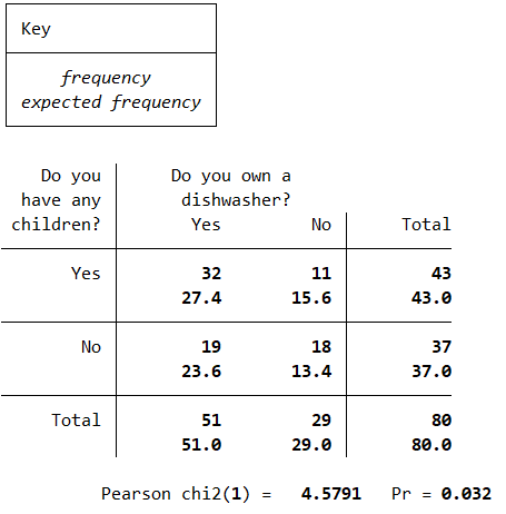
   tab q3 q16_3, chi2 expected
   

   The output for this command should be as follows:
   

   Note that in this case the expected frequencies are all greater than \(5\), but if the fifth assumption was violated you could conduct Fisher’s exact test using the following command instead:

   tab q3 q16_3, exact expected
   

5. The table for the chi-square test shows how the actual sample data compares with what would be expected if there was no association between having children and dishwasher ownership. The fact that there is a bit of a difference between the observed and expected values provides evidence of association in the sample, with the nature of the association being that people with children are more likely to own a dishwasher.

   To find out whether the association is significant, we need to refer to \(p\) value below the table. Since \(p < .05\) (in fact \(p = .032\)) we can reject the null hypothesis and conclude that there is a statistically significant association between having children and owning a dishwasher.

   For more information on how to interpret these results see the Introduction to statistics module.

Testing for linear correlation

A question you may wish to ask of the wider population is: Is there a statistically significant linear correlation between summer daily energy consumption and winter daily energy consumption?

This question can be answered by following the recommended steps, as follows:

1. The appropriate hypotheses for this question are:
   \(\textrm{H}_\textrm{0}\): There is no significant linear correlation between summer and winter daily energy consumption
   \(\textrm{H}_\textrm{A}\): There is significant linear correlation between summer and winter daily energy consumption

2. The appropriate test to use is Pearson’s correlation coefficient, as we are testing for linear correlation between two variables (summer daily energy consumption and winter daily energy consumption).

3. The assumptions for Pearson’s correlation coefficient are as follows:
   • Assumption 1: The sample is a random sample that is representative of the population.
   • Assumption 2: The observations are independent, meaning that measurements for one subject have no bearing on any other subject’s measurements.
   • Assumption 3: The variables are both continuous.
   • Assumption 4: Both variables are normally distributed, or the sample size is large enough to ensure normality of the sampling distribution.
   • Assumption 5: There is a linear relationship between the variables, as observed in the scatter plot (this is not strictly an assumption as Pearson’s correlation coefficient is still valid without it, but if you already know the relationship is not linear further interpretation is not necessary).
   • Assumption 6: There is a homoscedastic relationship between the variables (that is, variability in one variable is similar across all values of the other variable), as observed in the scatter plot (dots should be similar distance from line of best fit all the way along).

   While the first three assumptions should be met during the design and data collection phases, the fourth, fifth and sixth assumptions should be checked at this stage (for instructions on checking the normality assumption in Stata, see the The normal distribution page of this module).

   If the normality assumption is not met you can try transforming the data or using Spearman’s Rho or Kendall’s Tau-B instead. You can also use one of these tests if you have ordinal rather than continuous variables, or if there is non-linear correlation.

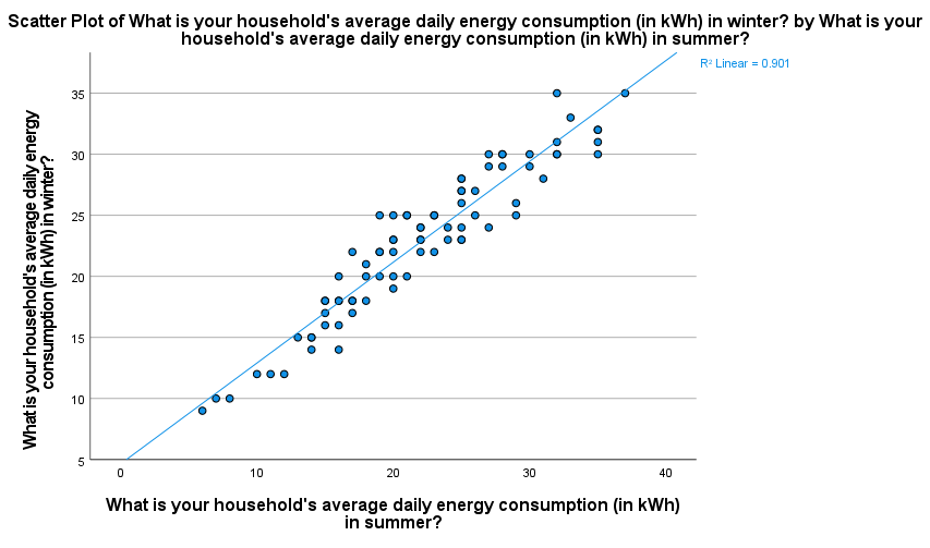
   To check for linearity and homoscedasticity, you can create a scatter plot with the independent variable on the \(x\)-axis and the dependent variable on the \(y\)-axis (for this example these are interchangeable; we will put summer consumption on the \(x\)-axis). For instructions on creating a scatterplot in Stata, see the Graphs page of this module.

   The scatterplot, with the line of best fit included, should look as follows. This shows that the relationship is approximately linear as the points lie close to the line of best fit. It also shows that the relationship is homoscedastic, as the points are a similar distance from the line of best fit all the way along (they don’t create a ‘funnel’ shape in either direction). Hence the fifth and sixth assumptions have been met.

   

4. If the assumptions are met, you can assess Pearson’s correlation coefficient in Stata by running the following command:

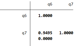
   pwcorr q6 q7, sig
   

   The output should look like this:

   

5. This table shows that Pearson’s correlation coefficient is \(.949\), indicating a strong positive linear correlation between summer and winter energy consumption (for more information on how to interpret this see the Descriptive statistics page of this module

   To test whether this linear correlation is statistically significant requires the \(p\) value (listed directly below the correlation coefficient). Since \(p < .05\) (in fact \(p < .001\)) we can reject the null hypothesis and conclude that there is a statistically significant linear correlation between summer energy consumption and winter energy consumption.

   Pearson’s correlation coefficient and its square (the coefficient of variation) are also measures of effect size, which can be used to test for practical significance. The correlation coefficient of \(.949\) indicates a large effect, and the coefficient of variation of \(90.06\%\) indicates that \(90.06\%\) of variation in winter energy consumption can be explained by variation in summer energy consumption.

   For more information on how to interpret these results see the Introduction to statistics module.