Introduction to Stata
Often when you are doing your analysis you will find that it is helpful to create new variables, or to make changes to existing variables. This page details three transformations which enable you to do this.
In brief, this page covers the following:
- How to compute a new variable using data from existing variables
- How to recode a categorical variable in order to create new categories for it
- How to convert a string variable to a numeric variable
- How to create categories for a continuous variable
Note that the examples covered make use of the Household energy consumption data.dta file, which contains fictitious data for 80 people based on a short ‘Household energy consumption’ questionnaire. If you want to work through the examples provided you can download the data file using the following link:
If you would like to read the sample questionnaire for which the data relates, you can do so using this link:
Also note that if you wish to save any of the output obtained from these examples, or any other output, you can create a log file.
Computing a new variable
Sometimes you may wish to create a new variable or variables to add to your data file, either from scratch or using the data from an existing variable or variables. For example, in the sample data file you may wish to create a new variable which gives the difference between summer and winter household energy consumption for each survey participant. You can do this using the generate command (which you can shorten to gen), specifying the name of the new variable and how it is to be calculated as follows:
gen Consumption_difference = q6 - q7
Once you have done this, you should see the name of the new variable appear in the Variables window at the top right of the screen. In addition, you can view or edit the data using the Data Editor window, and can edit the variable properties using the instructions provided in the Getting started page of this module.
As another example of when you might want to compute a new variable, consider questions q9 through q12, which all relate to satisfaction with different aspects of the participants’ electricity provider. As these questions all use the same rating system (measured on a scale of 1 to 5, with 1 indicating ‘Very unsatisfied’ and 5 indicating ‘Very satisfied’), the four variables representing these questions can be combined to come up with an overall satisfaction score.
One way of doing this is by adding all the variables together to create a score out of 20, which can be done using the gen command as follows:
gen overall_satisfaction = q9 + q10 + q11 + q12
If you run the tab command on this new variable (as described in the Descriptive statistics page of this module) you will see that there are only 78 satisfaction scores, whereas there are 80 cases in the data file. Looking at the actual data reveals why; the data in row 30 is missing for all four of the variables ‘q9’ to ‘q12’, and the data in row 31 is missing for variables ‘q10’ and ‘q12’. Since the numeric expression shown above only calculates new values for those cases that have complete data, the new variable has not been computed for rows 30 and 31.
Sometimes this will be what you want, but other times you will require data for the new variable regardless of whether some of the data is missing or not. To do this requires you to use the egen and row_total commands instead, as follows:
egen overall_satisfaction2 = rowtotal(q9 q10 q11 q12)
You may also like to experiment with other formulas. For example, if you wanted to calculate an average overall satisfaction score instead you could also try using two different, similar commands:
- The command gen average_satisfaction = (q9 + q10 + q11 + q12) / 4 will again have missing data for both rows 30 and 31.
- The command egen average_satisfaction = rowmean(q9 q10 q11 q12) will have missing data only for row 30. For row 31, the average will be calculated by dividing by 2 instead of 4, since there are only two variables with data.
Regardless of which formula you choose to use, the new variable can then be analysed in the usual way.
Recoding categorical variables
Sometimes you may wish to recode an existing categorical variable, most likely to reduce the number of categories by combining existing ones together. For example, in the sample data file you may wish to recode the ‘q8’ variable to reduce the number of categories from the current five to three (particularly as there are so few people in each category, and no-one in the ‘Strongly disagree’ category). You can do this using the recode command, and you can also add the generate (or gen) option if you would like to keep the existing variable and create a new variable, rather than overwriting the existing variable. For example, you can keep the existing ‘q8’ variable and create a new one which combines the existing categories into three as follows:
recode q8 (1/2=1) (3=2) (4/5=3), gen(q8_recoded)
Once you have done this, you should see the name of the new variable appear in the Variables window at the top right of the screen. In addition, you can view or edit the data using the Data Editor window, and can edit the variable properties using the instructions provided in the Getting started page of this module. In particular, you can assign labels to the new variable as follows:
label define q8_recoded_label 1 "Disagree" 2 "Neutral" 3 "Agree"
label values q8_recoded q8_recoded_label
Converting a string variable
Although Stata does allow alphabetic/string information to be entered as part of the data file, the more in-depth statistical analysis procedures require numeric data only (even if those numbers are simply codes or values representing categories).
At the questionnaire design stage it may be very difficult to anticipate the responses that will be given though, so creating a tick-box type question can be too complicated or restrictive. Hence allowing open-ended responses may be preferable instead, and the choice then is to either numerically code the data before keying it in, or to recode the responses once they have been entered into Stata. This section details how to do the latter, and uses the ‘q13’ variable in the sample data file as an example. This variable stores participant responses to the question:
What kind of hot water system do you use at your property?
The variable is a string variable, and running the tab command on it gives the following:
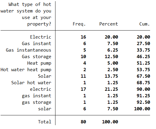
This output shows only five different types of hot water systems, but because of different spelling and terminology and different use of upper and lower case characters, twelve different responses are listed. To reduce this twelve down to the real five, the different categories need to be combined (that is, recoded).
To complete the first part of this two-step process requires use of the encode command, as follows:
encode q13, gen(q13_num)
This produces a new variable called ‘q13_num’, where the responses have been assigned to categories numbered from 1 to 12 (using a value label set also called ‘q13_num’).
The second step of the process is then to reduce these 12 categories to the 5 required ones, using the standard recode command. In this case, the existing and new categories could be as follows:
| Existing category | New category |
|---|---|
| 1 (electric) | 1 (Electric) |
| 2 (electric) | 1 (Electric) |
| 3 (gas instant) | 2 (Instantaneous gas) |
| 4 (Gas instant) | 2 (Instantaneous gas) |
| 5 (Gas instantaneous) | 2 (Instantaneous gas) |
| 6 (gas storage) | 3 (Gas storage) |
| 7 (Gas storage) | 3 (Gas storage) |
| 8 (Heat pump) | 4 (Heat pump) |
| 9 (Hot water heat pump) | 4 (Heat pump) |
| 10 (solar) | 5 (Solar) |
| 11 (Solar) | 5 (Solar) |
| 12 (Solar hot water) | 5 (Solar) |
Categorising continuous variables
Sometimes it is helpful to transform a continuous variable into a categorical variable, as this provides additional analysis options. For example, in the sample data file you may wish to transform the continuous ‘q1’ variable into categories, perhaps in order to make some comparisons for different age groups.
One way to do this is using the recode command as described in the previous section. For example, to make and label categories for people aged under 20, aged 20 to 29, aged 30 to 39 and aged 40 and above, you could type the following:
recode q1 (min/19=1) (20/29=2) (30/39=3) (40/max=4), gen(q1_grouped)
label define q1_grouped_label 1 "<= 19" 2 "20 - 29" 3 "30 - 39" 4 "40+"
label values q1_grouped q1_grouped_label
If your data has decimal places, however, you will need to think carefully about how you create your categories in order to ensure that no data is left out of them. If using the recode command to do this, some things to consider are that the ranges specified in the command are inclusive at both ends (for example, 20/29 includes both 20 and 29), and that if there are overlapping ranges the value will be assigned to the first matching range - so you may need to reorder the ranges in the command to account for this. Alternatively, you may find it easier to use the generate (or gen) and replace commands together instead. For example, you could create and label a second version of the previous variable as follows:
gen q1_grouped2 = .
replace q1_grouped2 = 1 if q1 < 20
replace q1_grouped2 = 2 if q1 >= 20 & q1 < 30
replace q1_grouped2 = 3 if q1 >= 30 & q1 < 40
replace q1_grouped2 = 4 if q1 >= 40 & q1 != .
label define q1_grouped_label2 1 "Age < 20" 2 "20 <= Age < 30" 3 "30 <= Age < 40" 4 "Age >= 40"
label values q1_grouped2 q1_grouped_label2
Once you have done this, you should see the name of the new variable(s) appear in the Variables window at the top right of the screen. In addition, you can view or edit the data using the Data Editor window, and can edit the variable properties using the instructions provided in the Getting started page of this module.