Microsoft Excel Essentials

The information on this page references the resource Party_Budget_Workbook_2 [XLSX, 11kB]. Download this workbook, if you haven’t already, and use it to work through the information below. This workbook has been formatted according to the instructions on the Getting started page of this module.

Another way you can summarise and analyse your data, this time without changing your source data, is through the use of pivot tables.

Creating a simple pivot table

To create a pivot table first highlight the data you wish to use; in this case we will highlight all data from cells A1 to F20. Alternatively, if your spreadsheet contains only source data, which it may in this case if you haven’t done any of the previous examples in this module, then you can click on any individual cell that contains data. Once you have done this, go to the Insert tab. You then have the option of creating a table out of your data first before creating a pivot table, which you should do if you plan to add more data later and you want to be able to automatically refresh your pivot table afterwards (once you have a pivot table you can do this by going to the Analyze tab, in PivotTable Tools, and choosing Refresh). If you do want to allow for this possibility, select Table and make sure the appropriate range of cells is selected, then click OK. You would then proceed to create a pivot table using the instructions that follow.

Since we are not going to be adding to our data we will instead go straight to PivotTable, where again you need to make sure that the appropriate range of cells is selected. You can also choose whether you want to create the pivot table in a new worksheet or in a specified location in the existing worksheet; we will do the former, so there is no need to change the default. Instead simply select OK, and then rename the new worksheet Item_Types.

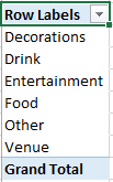
We will first create a simple pivot table in this worksheet listing all of the item types. To do this select TYPE from the list of fields on the PivotTable Fields pane on the right hand side of the worksheet (click in the specified area of the worksheet first if this pane is not displayed) and drag it to the ROWS area. The resulting pivot table should be as follows:

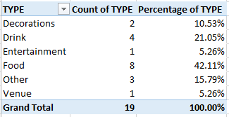
To add a count of the number of items of each type to this pivot table, select TYPE again and drag it to the VALUES area; a new column should be created in the pivot table showing how many items were purchased of each type. You may also want to add a column that displays these values as a percentage; to do this select TYPE and drag it to the VALUES area once again, and this time right click on one of the values in the new column. Then choose Show Values As → % of Grand Total. The values will now display as percentages (alternatively, rather than adding a new column we could have just adjusted the original count column in this way to show percentages instead).

Renaming column headings

At this point you might also want to rename the column headings so that they are more meaningful. You can do this by simply replacing the current headings with new headings of your choice manually, or you can switch to different automated headings by going to the Design tab (in PivotTable Tools), clicking on Report Layout and choosing either to Show in Outline Form or Show in Tabular Form. Do this now, and then also manually change the Count of TYPE2 heading to Percentage of TYPE. The resulting pivot table should look as follows:

Filtering

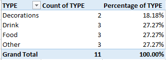
Once you have created your pivot table you can use it for further analysis if required. For example, you can filter the PivotTable to show the same information but for selected Suppliers; to do this select SUPPLIER and drag it to the FILTERS area. Then click the drop down arrow next to (All) and select one or multiple items to filter by (tick the Select Multiple Items box as required); try ticking Coles and Woolworths, for example, and check you get the following:

Once you have confirmed this, change the filter back to (All) again.

Adding another variable

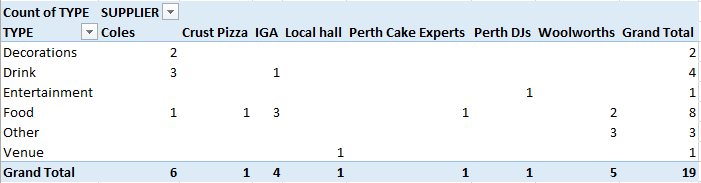
You can alter the pivot table to show how many of each type of item come from each supplier by having the suppliers in the columns of the table. Before we do this, first remove the percentage column from the table by clicking the drop down arrow for the Percentage of TYPE field in the VALUES area of the PivotTable Fields pane, and selecting Remove Field (if applicable). Now drag the SUPPLIERS field from the FILTERS area to the COLUMNS area, and the resulting pivot table should look as follows:

You can see the details of all items included in a particular count (or percentage) by double clicking on the count (or percentage) in the pivot table. Double click on the count of 2 for Decorations, for example, and a new worksheet should be created showing the details of the two decorations (i.e. Streamers and Balloons).

When you have finished creating pivot tables, navigate back to the Party_Budget sheet.