Microsoft Excel Essentials
Getting started in Excel generally means creating a new workbook, adding in your data, and then formatting your spreadsheet to help organise your data and make it more user friendly.
In brief, this page covers the following:
- How to create a new Excel workbook
- How to add headers to an Excel spreadsheet
- How to format cells in an Excel spreadsheet
- How to freeze panes in an Excel spreadsheet
- How to resize cells and wrap text in an Excel spreadsheet
- How to transpose data (that is, to swap data from rows to columns) in an Excel spreadsheet
This page provides instructions on how to create a new workbook, as well as the basic ways you can organise your document, including how to add and adjust headers, and how to format cells.
Creating a new workbook
When you open up Excel you will see that you have a range of preformatted documents to choose from. A blank workbook will most likely be the most common template that you will use, however you may like to experiment with other types as you continue using the software (note: a workbook refers to the whole Excel file/document, and the sheets are the separate pages you can use within that document).
In this module we will be using an existing workbook called Party_Budget, which you can download using the link below:
The spreadsheet in this workbook has been organised so that each column represents a field (category of information; in this case, name and type of item, supplier, cost and date paid) and each row represents a record (collection of information about a particular person, place, event or thing; in this case party expense). Where possible, you should ensure that you organise your data in the same way.
If you are working though certain pages or sections of this module and/or you do not want to format the document you can use this link instead:
The spreadsheet in this second workbook has already been formatted according to the guidelines on this page.
Adding headers
The data in the Party_Budget sheet currently does not have any headings. Let’s add some so that we can easily tell what data we are looking at. Firstly, we need to insert a new row. To do this, right click on the number 1 of your spreadsheet, and click Insert (you can also find insert options in the Cells section of the Home tab). Now that you have a new row, we can add our headings. From left to right, in separate cells, type the following:
ITEM
TYPE
SUPPLIER
AMOUNT_PAID
DATE_PAID
AMOUNT_OWING
Press the tab key or the left and right arrow keys to quickly move between cells.
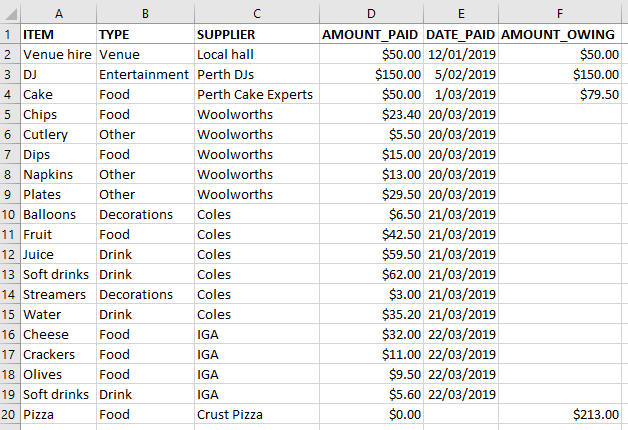
Your spreadsheet should now look like this:

You can format these headings so that they stand out from the rest of the data by changing the style (e.g. bold, italic), colour, and background fill. These options can all be found in the Font section of the Home tab. Play around with them to get your sheet looking how you want it.
At this point it is worth noting that many of these formatting changes will only be recognised by humans, and that there are limits to what Excel will pick up on. For example, while you can sort or filter your data according to cell or font colour, it is usually quite difficult to write formulas that take into account these things. Hence while it is fine to format your sheets to make them nicer for humans to look at, just make sure that anything that needs to be machine readable (i.e. understood by Excel or other software) is (for example, by including separate columns for each field as in the Party_Budget spreadsheet as needed, rather than just colour coding the items).
Machine readability is also the reason the headings used above have underscores in them rather than spaces, as some software does not recognise these. If the data is just for use in Excel then there is no need to be so concerned about this, but if there is a chance your data may eventually be used in other software then you should follow the convention of using only letters, numbers, underscores, and dashes in any file, field, or header names you create.
Formatting cells
You can format cells depending on what type of information they contain or will contain. For instance, in columns D and F are a list of prices to one decimal place. To format these as currency select both columns by holding down the Ctrl button and clicking on the D and the F at the same time. Then right-click anywhere in either of the columns and select Format Cells. You will then see a list of options to choose from, including General, Number, Currency, and so on. Select Currency and click OK. The numbers in both lists will now be formatted as dollar amounts to two decimal places.
Freezing panes
Sometimes, when you’re working with a large data set, it’s useful to be able to keep the category or heading panes in view as you navigate the set. To do this you will need to “freeze” the panes, which you can do by going to the View tab, selecting Freeze Panes and then Freeze top row. You will also see options there for if you wanted to freeze a selected section of cells, or freeze the first column.
Resizing cells and wrapping text
You will notice that some of the data in the sheet appears to be cut-off:
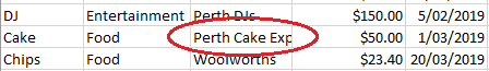
There are a few ways to expand the columns so that the text fits. The first is to hover over the line between the column your text is in and the one after it (C and D in this case, as pictured below), and double-click when the two-way arrow comes up:

This will expand the C column to the width of the largest piece of data (e.g. “Perth Cake Experts”). You can also click and drag on the two-way arrow to adjust the column to the width you want. If you have multiple columns that need resizing you can do them at the same time by highlighting all the relevant column headers (do this using Ctrl if they are not adjacent), then hovering over the end of one of the columns so that the two-way arrow appears and double-clicking or dragging to the desired width.
Another option you can choose to display your text is to wrap it. To do this select the cells, rows or columns you want to wrap, go to the Home tab and in the Alignment section select Wrap Text. Now if you add more text to a cell it will stay at the width you have selected, but will be shown on a new line within the same cell, rather than being cut off or hidden.
After formatting your document, your spreadsheet will look like this:
Transposing data
Occasionally you might find that you wish to transpose your data; that is, change the columns of your spreadsheet to rows and vice versa. To do this, highlight the data you would like to transpose, (e.g. all of the Party_Budget data), and copy it (by right-clicking and selecting Copy or by pressing Ctrl + C). Next, choose where you would like to paste the transposed data (try adding a new sheet and renaming it, e.g. to Transposed_Data), then right-click on the cell in the top left-hand corner of where you would like to paste it (the A1 cell in your new sheet for example) and choose Transpose (T) from the Paste Options. That option looks like this:
![]()
Your data will be transposed, with the columns as rows and the rows as columns. It may look a little scary, with a row containing a lot of # symbols:
![]()
You just need to resize the columns to fit the data, in particular to view the dates in this example:
![]()
Don’t worry too much about formatting this spreadsheet now though as we will continue to use the original Party_Budget sheet for the remainder of the module, so ensure you have selected it again before moving on.