Microsoft Excel Essentials
One of Excel’s key features is the ability to use formulas and functions to analyse and manipulate data.
In brief, this page covers the following:
- How to write formulas to perform calculations in Excel
- The different reference types you can use in Excel formulas
- An overview of Excel’s built-in functions
- The AVERAGE, COUNT and SUM AutoSum functions
- The AND, IF and OR logical functions
- The XLOOKUP function
Note that the information on this page references the resource Party_Budget_Workbook_2 [XLSX, 11kB]. Download this workbook, if you haven’t already, and use it to work through the information below. This workbook has been formatted according to the instructions on the Getting started page of this module.
Formulas
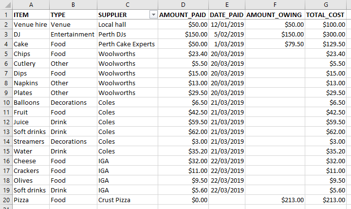
You can create formulas in Excel to perform calculations, typically by referring to values in cells in your workbook. For example, we can add together the amounts paid and amounts owing to find the total cost of each item in the list using formulas. We will do this in column G, which you should first give the heading TOTAL_COST. Now click on cell G2 and type the = sign, then either select cell D2 or type D2, type the + sign and finally either select cell F2 or type F2. Pressing Enter should then give you the total cost, which is $100 in this case. If it doesn’t, check that you have entered the formula correctly by clicking on the cell where you entered it (ie. G2) and looking at the formula bar:

You can always make edits to the formula in the formula bar if you need to.
Reference types
Something important to note when creating formulas in Excel is the different reference types. The default in Excel is a relative reference, meaning that any references to cells you make in your formula are relative to the location of the cell where the formula is. For example, the formula that we have just written is a formula that refers to the cells three places and one place to the left of it respectively. If we copy and paste the formula in cell G3, for example, the formula adds together the values in cells D3 and F3 instead to give a total cost of $300. This is very useful in instances such as this, when we are wanting to perform the same operation for different sets of cells. Indeed, we can now copy the formula to the rest of the cells in the TOTAL_COST column to find the total cost of the remaining items by clicking on cell G3, hovering the mouse over the bottom-right corner of the cell until the black + symbol shows, and double clicking. Doing this should make the page look like this:
Alternatively, if you want the formula to remain exactly the same in the new cell you are copying it to you need an absolute reference. You can convert to this reference type by either manually adding $ signs to the front of all the column and row references in the formula bar, or by highlighting it in the formula bar and clicking F4. Try doing this to the formula in cell G20:

If you then press Enter and copy and paste the formula in cell I2, for example, the result should be the same total of $213 (delete the value in cell I2 when you have confirmed this).
Finally, you might sometimes want to use a mixed reference to keep either the row or the column absolute, but the other relative. You can do this by typing the $ sign only in front of either the row or the column reference as appropriate, or by highlighting the formula and pressing F4 until you have the desired result.
Built-in functions
For anything beyond the simple calculations described above, making use of Excel’s built-in functions in your formulas is a must. The following sections outline a few of the most commonly used ones, but there are hundreds to choose from. You can find them by going to the Formulas tab and browsing through the lists of functions grouped into various categories, or by selecting Insert Function and searching for a function using a brief description. Either way, you can see details of the pieces of information (known as arguments) that are required to be entered as part of the function, and can click on Help on this Function for a detailed description of it if required. Alternatively, if you are not sure of the exact name of a function but know what it starts with you can type the = sign in a cell and then start typing to see a list of functions, which you can then select from by double clicking. You can also find a list of all functions, along with detailed descriptions, on this Microsoft Support page link.
AutoSum functions
The AVERAGE, COUNT and SUM functions are three commonly used functions when working with numbers. They are as follows:
AVERAGE finds the average (mean) of values. It takes up to 255 arguments, which can be numbers, cell references, or ranges.
COUNT counts how many values are numbers. It takes up to 255 arguments, which can be items, cell references, or ranges.
SUM adds values together. It takes up to 255 arguments, which can be numbers, cell references, or ranges.
Each of these functions can be performed by typing the function as part of a formula or by using AutoSum or Quick Analysis. To type the AVERAGE function to average all the amounts paid, for example, first select the cell where you want the average displayed. Do this in cell D21 by typing the following (or at least start typing it, then double-click on the name of the function when it appears):
=AVERAGE(
You can then average the values in the column either by entering all the cell references as individual arguments or, more efficiently, by entering the range of cell references as a single argument (recommended). To do the latter either type D2:D20 or highlight the relevant cells D2 to D20; either way, the result when you press Enter should be $31.75 and the formula should look like this:

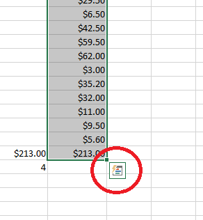
To use AutoSum to perform the COUNT function to count of the number of items that still have amounts owing, for example, highlight cells F2 to F20 then click on the Formulas tab, select AutoSum and choose Count Numbers. A count of the total amount of numbers in the highlighted cells will appear in cell F21, although as this entire column was previously formatted as currency it appears as $4.00. To change the value to 4, which is the number of items still requiring some payment, simply reformat the cell as General using the method described previously. To use Quick Analysis to perform the SUM function to add together all of the total costs, for example, highlight cells G2 to G20 then click on the Quick Analysis icon in the bottom right hand corner:
Select the Totals tab and choose Sum, and the sum of $1095.70 should appear in cell G21. You can edit any formulas created using AutoSum or Quick Analysis in the formula bar if needed.
Logical functions
Logical functions, which check conditions and return results accordingly, are further examples of commonly used functions in Excel. Three examples of such functions are AND, IF and OR, which are often used together. Each function is as follows:
AND checks multiple conditions at the same time. It takes up to 255 arguments, which are the conditions, and returns TRUE if they are all true and FALSE if they are not.
IF makes a logical comparison and returns a value depending on the result. It takes three arguments; the logical expression to be evaluated (which can include AND, OR functions), the value to return when the expression is TRUE, and the value to return when the expression is FALSE.
OR checks multiple conditions at the same time. It takes up to 255 arguments, which are the conditions, and returns TRUE if any of them are true and FALSE if they are not.
As an example of using the IF and OR functions together, consider that we want to categorise the items in the list to see which ones were purchased from a supermarket and which were not. We will do this in column H, which you should first give the heading SUPPLIER_TYPE. Now click on cell H2 and type the following (or at least start typing it, then double-click on the name of the function when it appears):
=IF(
You then need to enter three arguments, the first of which is the logical test. In this case this requires use of the OR function, as you need to check whether the supplier is Woolworths or Coles or IGA (i.e. if it is any of the supermarkets). So the first argument, which you can create by typing or by a combination of typing and selecting cell C2, should be as follows:
OR(C2 = “Woolworths”, C2 = “Coles”, C2 = “IGA”)
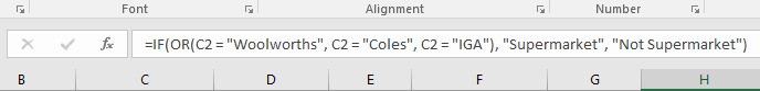
The second and third arguments of the IF function will then be the values you wish to return if this is TRUE or FALSE respectively (it will be TRUE if any of the three conditions are TRUE, and FALSE if they aren’t). So enter a comma and a space after your previous argument and then type “Supermarket”, a comma and a space, and “Not supermarket”, for example. be sure to add a closing bracket at the end. When you press Enter the value in the cell should read ‘Not supermarket’, as this item was not purchased from a supermarket, and the formula should look like this:
Copy this relative reference to the rest of the cells in the Supplier Type column to find the supplier type of the remaining items by clicking on cell H2, hovering the mouse over the bottom-right corner of the cell until the black + symbol shows, and double clicking.
As another example, consider that you can use the AND and IF functions together to indicate which supermarket items cost more than $20. Do this in cell I2 by typing the following formula, which checks whether an item was purchased from a supermarket (using the new value in cell H2) and cost more than $20 (using the total cost in cell G2), and returns text if it was and no text if it wasn’t:
=IF(AND(H2= “Supermarket”, G2 > 20), “Supermarket item more than $20”, “”)
Again, you can copy this relative reference to the rest of the cells in column I to see the result for all items in the list.
Finally, three variations of the IF function that may be of interest are the AVERAGEIF, COUNTIF and SUMIF functions. Each of these functions test if cells in a certain range (the function’s first argument) meet a set criteria (the function’s second argument) and average, count or sum, respectively, those that do. For example, typing the following formula in cell B21 will count the number of items in the list that have been categorised as Food in the TYPE column:
=COUNTIF(B2:B20, “Food”)
This formula should give the result of 8.
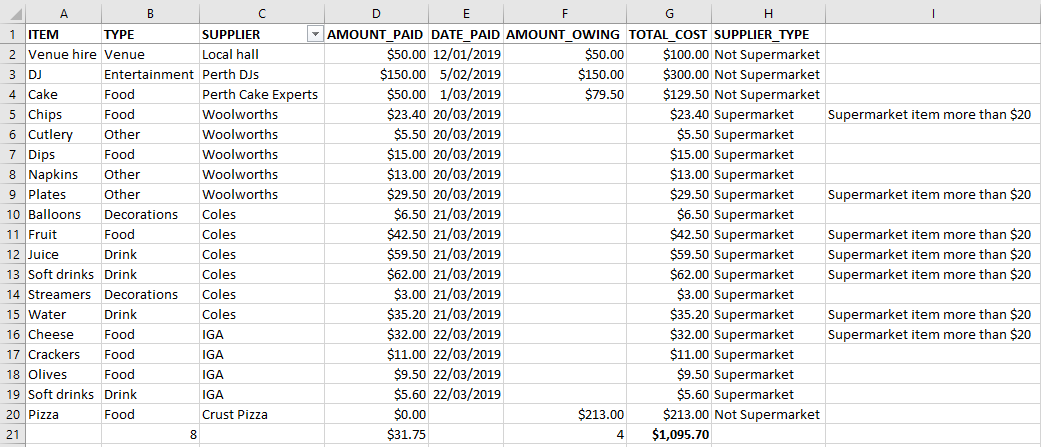
If you’ve completed all the previous pages of this module, at the end of this page your spreadsheet should look something like this:
XLOOKUP
The function XLOOKUP can be useful when you want to look things up in a spreadsheet. XLOOKUP replaces the old VLOOKUP and HLOOKUP since it can be used when your data is arranged either vertically or horizontally.
The XLOOKUP function has six possible arguments to add to the formula. Before you fill them out, the formula will look like this:

The first three arguments are required. The other three, in the square brackets, are optional. Whether you use them will depend on your needs and what you are searching for.
lookup_value: this is the value you want to look up.
lookup_array: this is the range of cells that make up the search area, or the search area that your lookup_value should be in.
return_array: this is the range of cells that make up the area of the result that we want, or the search area where your result will be. This range of cells can be anywhere in your spreadsheet, or even in another sheet within your workbook.
[if_not_found]: this is what will be returned if your lookup_value doesn’t exist in your lookup_array. The default return is #N/A, but you can set an if_not_found argument to make the return whatever you like, including text if you put the text into double quotation marks, “…”. However, this will be affected by the formatting of your cells.
[match_mode]: this specifies the type of match you will get. The XLOOKUP function will look for an exact match if this argument is not included in your formula. However, you can use the match_mode argument to return a similar match if an exact match can’t be found. Click on the match_mode argument in the formula in excel for additional options.
[search_mode]: this allows your search to be performed in different ways. The default search mode is to search from the first value, and this is what the function will do if you don’t input a value for this argument into the formula. You can change this so that the search is performed in reverse, or a binary search is performed. Click on the argument in the formula in excel for additional options.
As an example, consider that we want to find out the date we paid for fruit for the party. To use XLOOKUP for this we first need to choose the cell where the result is to be displayed. Use B22 for example, although note you should first format this cell as a Date, using the method described in the Getting started page of this module, to ensure that the value displays correctly for this particular example. You may also want to type the word Fruit in cell A22, to show that this is the item the date refers to (you can also use this to help in step 1 below). Now click in cell B22 and type the following (or at least start typing it, then double-click on the name of the function when it appears):
=XLOOKUP(
You will then be prompted to enter at least three arguments as follows:
lookup_value: in this case we want to find out the date we paid for the fruit, so “Fruit” is our lookup_value. We can enter it like this (i.e. in quotes), or if you have typed Fruit in cell A22 then just click on that cell and the cell reference will appear as part of the function.
lookup_array: we are searching for the item ‘Fruit’, so our search area is column A, or A2 to A20. You can either enter A2:A20 in the formula, or highlight all the values in the column by selecting A2 and dragging down, or selecting the cell A2 and using Control, Shift and Down on your keyboard to highlight all the relevant cells.
return_array: In this case, we want to know the date that we paid for the fruit. Our return_array will be all the values in column E, the DATE_PAID column. However, we also need to include the blank E20 cell, as the lookup_array and the return_array need to be the same size for XLOOKUP to work.
For this example, we don’t need to add anything for the last three arguments, the default settings will work. So, the formula will look like this:

or like this:

Now press Enter and your XLOOKUP should return the result 21/03/2019 as the date the fruit was paid for in this case.
As another example, let’s say we had to hire more chairs for the party and we wanted to know if they’ve been included in the list and if so, who’s supplying them. Type the word Chairs into A23, and then in cell B23 start typing the XLOOKUP formula again.
This time your lookup_value will be A23, or “Chairs”.
Your lookup_array will be A2:A20 again.
And your range_array will be E2:E20 again.
As we aren’t sure about whether chairs have been included yet, let’s also add an if_not_found argument. You can make this anything you want. For example, “Haven’t enquired yet”.
Now press Enter and your XLOOKUP should return the result Haven’t enquired yet. If it doesn’t check that your formula looks like this:

If we didn’t add an argument for if_not_found the XLOOKUP would have returned #N/A as a result.
Note that a limitation of XLOOKUP is that if the lookup_value occurs more than once, a result is only returned for the first occurrence. For example, if we wanted to search for who was supplying the soft drinks, it would only provide the output of Coles as that is the first occurrence. If we used -1 in the search_mode argument to reverse the search and start at the last item, XLOOKUP would return IGA as the supplier, since that is the first occurrence starting from the last item. However, it will still only return the one value.