Introduction to Stata

Many of the statistics detailed in the Inferential statistics page of this module rely on the assumption that continuous data approximates a normal distribution, or that the sample size is large enough that the sampling distribution of the mean approximates a normal distribution. This page details how to use Stata to test whether a continuous variable is normally distributed, while the Introduction to statistics module provides more information about what the normal distribution is and when testing for it is required.

Note that the examples covered make use of the Household energy consumption data.dta file, which contains fictitious data for 80 people based on a short ‘Household energy consumption’ questionnaire. If you want to work through the examples provided you can download the data file using the following link:

• Household energy consumption data [DTA, 25kB]

If you would like to read the sample questionnaire for which the data relates, you can do so using this link:

• Household energy consumption questionnaire [PDF, 187kB]

Also note that if you wish to save any of the output obtained from these examples, or any other output, you can create a log file.

Testing for normality

As explained in the Introduction to statistics module, it is helpful to consult a number of different measures in order to make a decision about normality. You can use a series of commands in Stata to obtain the required output.

For example, to test whether the ‘q6’ variable (which measures average daily summer energy consumption in kWh in the sample data file) is normally distributed, run the following:

sum q6, detail
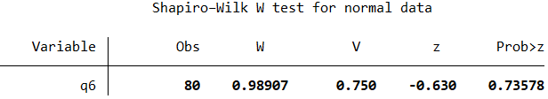
swilk q6
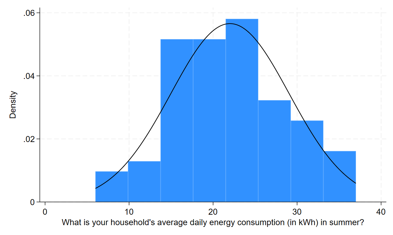
histogram q6, normal name(histogram_q6, replace)
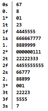
stem q6
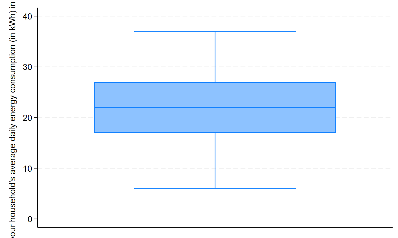
graph box q6, name(boxplot_q6, replace)
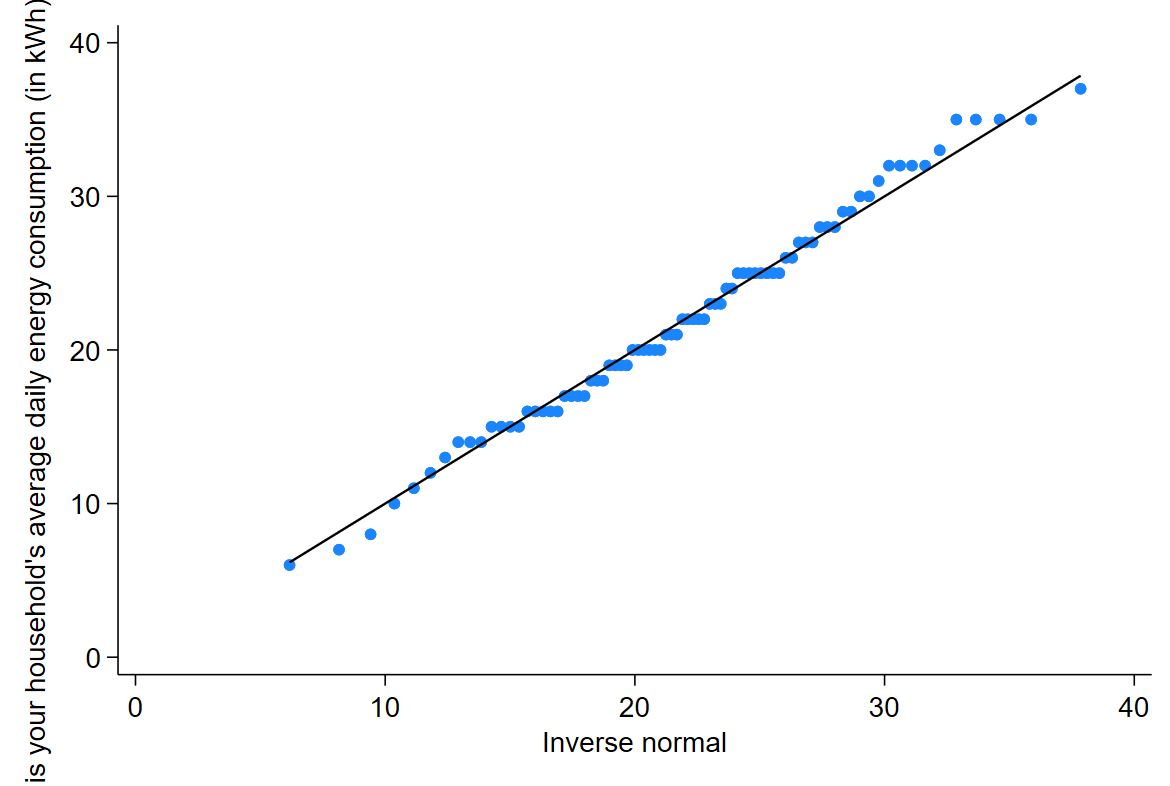
qnorm q6, name(normalQQ_q6, replace)

The output should be as follows (use the graph display command to view the required graphs, as detailed in the Graphs page of this module):

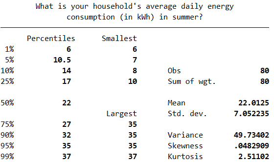
This output can then be evaluated as explained in the Introduction to statistics module. In particular, you should observe the following:

• The mean and median (as shown in the first table) are extremely similar. Note that if you would also like to compare the mode, you can obtain this as detailed in the Descriptive statistics page of this module. While this is a bit higher, at \(25\), this is less of a concern.

• The skewness is \(0.048\) (as shown in the first table), which is well within the acceptable range of \(-1\) to \(1\)

• The kurtosis is \(2.51\) (as shown in the first table), which is within the acceptable range of \(2\) to \(4\) (note that Stata provides the value for actual kurtosis, rather than excess kurtosis, which ideally should be 3 but can be anywhere within this range)

• The \(p\) value for the Shapiro-Wilk test is \(.736\) (as listed under ‘Prob>z’ in the second table), which is greater than \(.05\) as required.

• The histogram is roughly symmetrical.

• The stem and leaf plot is roughly symmetrical.

• The points do not deviate much from the line in the Normal Q-Q plot.

• The median is approximately in the middle of the box plot, the whiskers are of similar length and there are no outliers.

Hence it can be concluded that the ‘q6’ variable is approximately normally distributed.

Transforming variables

If you find that a variable is not normally distributed when you require it to be, you can try transforming the variable to see if this makes it better approximate a normal distribution. Some examples of transformations to try are provided in the Introduction to statistics module.

You can apply any of these transformations by generating a new variable using the gen command, as described in the Transformations page of this module. Once you have done this, you will need to test again for normality in the usual way.

Testing for normality in two or more groups

Sometimes rather than testing that all of a continuous variable’s data is normally distributed, you need to check that the continuous variable’s data is normally distributed for each category of a categorical variable. In future you may want to write a loop in Stata to do this, but in the meantime probably the easiest option is to adapt the previous normality commands to filter for each category manually.

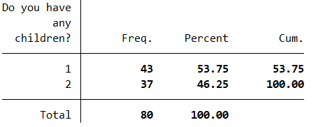
For example, to test whether the ‘q6’ variable (which measures average daily summer energy consumption in kWh in the sample data file) is normally distributed for each group of the ‘q3’ variable (which shows whether or not the participant has any children in the sample data file), you should first establish the category numbers used. One way of doing this is as follows:

tab q3, nolabel

The output from this command should be as follows:

Next, you can use these category numbers to run the normality commands for each category separately, as follows:

sum q6 if q3 == 1, detail
swilk q6 if q3 == 1
histogram q6 if q3 == 1, normal name(histogram_q6_q3_1, replace)
stem q6 if q3 == 1
graph box q6 if q3 == 1, name(boxplot_q6_q3_1, replace)
qnorm q6 if q3 == 1, name(normalQQ_q6_q3_1, replace)

sum q6 if q3 == 2, detail
swilk q6 if q3 == 2
histogram q6 if q3 == 2, normal name(histogram_q6_q3_2, replace)
stem q6 if q3 == 2
graph box q6 if q3 == 2, name(boxplot_q6_q3_2, replace)
qnorm q6 if q3 == 2, name(normalQQ_q6_q3_2, replace)

The output will be very similar to the output obtained without filtering, but this time there will be a set of statistics and graphs for each group. These should be analysed separately, and you may sometimes find that the data is normally distributed for all groups, for some groups only, or for none of the groups. In this case, the output indicates that the ‘q6’ variable is normally distributed for both the group that has children, and the group that doesn’t.