Introduction to Stata

There are two key types of inferential statistics, estimation and hypothesis testing, and Stata can be used to assist with both. This page looks at confidence intervals and at the fundamentals of hypothesis testing with regards to Stata, while subsequent pages of the module focus on how to conduct some common inferential statistical tests in Stata. Alternatively, for more information on inferential statistics you may like to visit the Introduction to statistics module.

Note that the examples covered make use of the Household energy consumption data.dta file, which contains fictitious data for 80 people based on a short ‘Household energy consumption’ questionnaire. If you want to work through the examples provided you can download the data file using the following link:

• Household energy consumption data [DTA, 25kB]

If you would like to read the sample questionnaire for which the data relates, you can do so using this link:

• Household energy consumption questionnaire [PDF, 187kB]

Also note that if you wish to save any of the output obtained from these examples, or any other output, you can create a log file.

Determining a confidence interval

A confidence interval is a range of probable values for an unknown population parameter, based on the sample statistic (for example the mean). The percentage associated with the confidence interval is termed the confidence coefficient, and this is the level of confidence you have that the range actually includes the true value. Stata automatically calculates confidence intervals for a range of statistics, with the default being a \(95\%\) confidence interval. For example, the following details how to obtain and interpret a \(95\%\) confidence interval for the mean of a continuous variable. If you would like more information on confidence intervals you may first like to visit the Introduction to statistics module.

A question you may wish to ask of the data is: Based on the data observed in the sample, what is the \(95\%\) confidence interval for the population mean summer energy consumption?

Before calculating this confidence interval in Stata, it is important to note that some assumptions need to be met when using a confidence interval to estimate the mean of a population. These assumptions are as follows:

• Assumption 1: The sample is a random sample that is representative of the population.

• Assumption 2: The observations are independent, meaning that measurements for one subject have no bearing on any other subject’s measurements.

• Assumption 3: The variable is normally distributed, or the sample size is large enough that the sampling distribution of the mean approximates a normal distribution.

While these first two assumptions should be met during the design and data collection phases, the third assumption should be checked at this stage. For instructions on testing for normality in Stata, see the The normal distribution page of this module.

If all assumptions are met (as is the case for this example), you can obtain a \(95\%\) confidence interval for the mean in Stata by using the mean command as follows:

mean q6

The output should be as follows:

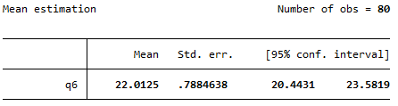
This tells us that based on what has been observed in the sample, we can be \(95\%\) confident that the mean summer energy consumption of the wider population is somewhere between \(20.44\) kWh (lower bound) and \(23.58\) kWh (upper bound).

Note that to calculate a confidence interval for the mean with a confidence coefficient other than \(95\%\), you can add the level option after a comma with the required confidence coefficient in brackets. For example:

mean q6, level(99)

Hypothesis testing

Hypothesis testing involves testing statements (hypotheses) about the population using data collected in the sample. The particular test to use depends on the nature of the hypothesis, and there are often versions of each test that are parametric (assume normal distribution and require at least one continuous variable) and non-parametric (don’t assume normal distribution and can be used for ordinal variables). If you would like more information on hypothesis testing, you may like to visit the Introduction to statistics module.

Some common examples of hypothesis tests are one sample, paired samples and independent samples \(t\) tests, one-way ANOVA, the chi-square test of independence and Pearson’s correlation (all of which are covered in later pages of this module). Whichever test you are using, it is important to note that conducting the test in Stata is just part of the process. In particular, the recommended steps to follow in order to successfully conduct a hypothesis test are listed below.

1. Determine the hypothesis to be tested.
2. Establish the appropriate test for the hypothesis.
3. Check that all assumptions for the test are valid (Stata can help with some of these).
4. Use Stata to conduct the relevant test and determine the \(p\) value and confidence interval (if applicable).
5. Interpret the result.

Examples of how to do this for each of the tests in the table are covered in the following pages.