Introduction to Stata
One of the reasons you may wish to do a hypothesis test is to determine whether there is a statistically significant difference between means, either for a single sample (in which case you would compare to a constant value) or for multiple independent or related samples (in which case you would compare between these different samples). Depending on the exact nature of the analysis, different tests are required, and this page details the process for performing some of the most common ones using Stata.
In brief, it covers how to do the following in Stata:
- Conduct and interpret the output for a one sample \(t\) test
- Conduct and interpret the output for a paired samples \(t\) test
- Conduct and interpret the output for an independent samples \(t\) test
- Conduct and interpret the output for a one-way ANOVA
Note that the examples covered make use of the Household energy consumption data.dta file, which contains fictitious data for 80 people based on a short ‘Household energy consumption’ questionnaire. If you want to work through the examples provided you can download the data file using the following link:
If you would like to read the sample questionnaire for which the data relates, you can do so using this link:
Also note that if you wish to save any of the output obtained from these examples, or any other output, you can create a log file.
Conducting a one sample \(t\) test
A question you may wish to ask of the wider population is: Does this sample come from a population where the mean summer daily energy consumption is \(19\)kWh
This question can be answered by following the recommended steps, as follows:
-
The appropriate hypotheses for this question are:
\(\textrm{H}_\textrm{0}\): The sample comes from a population with a mean summer daily energy consumption of \(19\)kWh
\(\textrm{H}_\textrm{A}\): The sample does not come from a population with a mean summer daily energy consumption of \(19\)kWh -
The appropriate test to use is the one sample \(t\) test, as we are testing whether the sample comes from a population with a specific mean (\(19\)kWh in this case).
- The assumptions for a one sample \(t\) test are as follows:
- Assumption 1: The sample is a random sample that is representative of the population.
- Assumption 2: The observations are independent, meaning that measurements for one subject have no bearing on any other subject’s measurements.
- Assumption 3: The variable is continuous.
- Assumption 4: The variable is normally distributed, or the sample size is large enough to ensure normality of the sampling distribution.
While the first three assumptions should be met during the design and data collection phases, the fourth assumption should be checked at this stage (for instructions on doing this in Stata, see the The normal distribution page of this module). If the normality assumption is not met you can try transforming the data or conducting the One sample Wilcoxon signed-rank test instead (you can also use this test if you have an ordinal rather than continuous variable).
-
If all the assumptions are met you can conduct the one sample \(t\) test in Stata using the ttest command as follows:
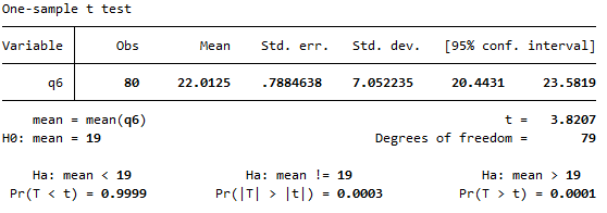
ttest q6 == 19The output should look like this:
-
From the table we can see that the mean summer daily energy consumption in our sample is \(22.01\)kWh, which is \(3.01\)kWh more than our hypothesised value. To test whether this is a statistically significant difference, we need to refer to the \(p\) value and confidence interval.
While there are actually three \(p\) values listed below the table, the standard one to use is the middle one, which is the two-tailed \(p\) value. This is used to test for a difference in either direction (that is, to test whether the mean is significantly greater than or less than \(19\), as per our alternative hypothesis). Since \(p < .05\) (in fact \(p = 0.0003\)) and since the \(95\%\) confidence interval for the population mean summer daily energy consumption does not include the value of \(19\) (\(95\% \textrm{CI}\) [\(20.4431\)kWh, \(23.5819\)kWh]), we can reject the null hypothesis and conclude that the sample actually comes from a population with mean summer daily energy consumption significantly more than \(19\)kWh.
For more information on how to interpret these results see the Introduction to statistics module.
Conducting a paired samples \(t\) test
A question you may wish to ask of the wider population is: Is there a statistically significant difference between mean summer daily energy consumption and mean winter daily energy consumption?
This question can be answered by following the recommended steps, as follows:
-
The appropriate hypotheses for this question are:
\(\textrm{H}_\textrm{0}\): There is no significant difference between mean summer and winter daily energy consumption
\(\textrm{H}_\textrm{A}\): There is a significant difference between mean summer and winter daily energy consumption -
The appropriate test to use is the paired samples \(t\) test, as we are comparing the means of two related groups (summer and winter consumption for the sample people).
- The assumptions for a paired samples \(t\) test are as follows:
- Assumption 1: The sample is a random sample that is representative of the population.
- Assumption 2: The observations are independent, meaning that measurements for one subject have no bearing on any other subject’s measurements.
- Assumption 3: The variables are both continuous.
- Assumption 4: Both variables as well as the difference variable (the differences between each data pair) are normally distributed, or the sample size is large enough to ensure normality of the sampling distributions.
While the first three assumptions should be met during the design and data collection phases, the fourth assumption should be checked at this stage (for instructions on doing this in Stata, see the The normal distribution and Transformations pages of this module). If the normality assumption is not met you can try transforming the data or conducting the Wilcoxon signed rank test instead. You can also use this test if you have ordinal rather than continuous variables.
-
If all the assumptions are met you can conduct the paired samples \(t\) test in Stata in Stata using the ttest command as follows:
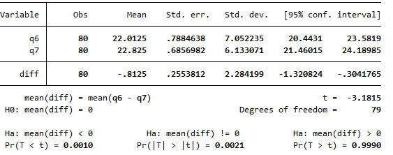
ttest q6 == q7The output should look like this:
-
From the table we can see that the mean summer daily energy consumption in our sample is \(22.01\)kWh, while the mean winter daily energy consumption is \(22.83\)kWh; a difference of \(0.81\)kWh. To test whether this is a statistically significant difference, we need to refer to the \(p\) value and confidence interval.
While there are actually three \(p\) values listed below the table, the standard one to use is the middle one, which is the two-tailed \(p\) value. This is used to test for a difference in either direction (that is, to test whether one mean is significantly greater than or less than the other, as per our alternative hypothesis). Since \(p < .05\) (in fact \(p= .0021\)) and since the \(95\%\) confidence interval for the difference between the population mean summer and winter daily energy consumptions does not include zero (\(95\% \textrm{CI}\) [\(-1.321\)kWh, \(-0.304\)kWh]), we can reject the null hypothesis and conclude that the mean summer daily energy consumption is significantly less than the mean winter daily energy consumption.
For more information on how to interpret these results see the Introduction to statistics module.
Conducting an independent samples \(t\) test
A question you may wish to ask of the wider population is: Is there a statistically significant difference in mean summer daily energy consumption for those with and without children?
This question can be answered by following the recommended steps, as follows:
-
The appropriate hypotheses for this question are:
\(\textrm{H}_\textrm{0}\): There is no significant difference in mean summer daily energy consumption for those with and without children
\(\textrm{H}_\textrm{A}\): There is a significant difference in mean summer daily energy consumption for those with and without children -
The appropriate test to use an independent samples \(t\) test, as we are comparing the means of two unrelated groups (summer consumption of those with and without children).
- The assumptions for an independent samples \(t\) test are as follows:
- Assumption 1: The sample is a random sample that is representative of the population.
- Assumption 2: The observations are independent, meaning that measurements for one subject have no bearing on any other subject’s measurements.
- Assumption 3: The dependent variable is continuous.
- Assumption 4: The variable is normally distributed for both groups, or the sample size is large enough to ensure normality of the sampling distribution.
While the first three assumptions should be met during the design and data collection phases, the fourth assumption should be checked at this stage (for instructions on doing this in Stata, see the The normal distribution page of this module). If the normality assumption is not met you can try transforming the data or conducting the Mann-Whitney U test instead. You can also use this test if you have an ordinal rather than continuous dependent variable.
-
If all the assumptions are met you can conduct the independent samples \(t\) test in Stata. However, first you may want to run Levene’s Test for Equality of Variances to check whether the group variances are equal. You can do this using the robvar command, as follows:
robvar q6, by(q3)The output should look like this:
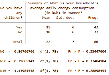
The \(p\) value for Levene’s Test for Equality of Variances (listed in the first row below the table, after \(Pr > F =\)) is \(p > .05\) (in fact \(p = .354\)), so we can assume equal variances. In this case you would run the independent samples \(t\) test using the ttest command as follows (note that if the variances were not equal, you would add unequal directly after this command):
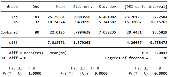
ttest q6, by(q3)The output should look like this:
-
From the table we can see that the mean summer daily energy consumption in our sample for those with children is \(25.26\)kWh, while for those without children it is \(18.24\)kWh; a difference of \(7.01\)kWh. To test whether this is a statistically significant difference, we need to refer to the \(p\) value and confidence interval.
While there are actually three \(p\) values listed below the table, the standard one to use is the middle one, which is the two-tailed \(p\) value. This is used to test for a difference in either direction (that is, to test whether one mean is significantly greater than or less than the other, as per our alternative hypothesis). Since \(p < .05\) (in fact \(p= .0000\), which doesn’t mean that \(p\) is actually zero but that it is very very small) and since the \(95\%\) confidence interval for the difference between the population mean summer daily energy consumptions of those with and without children does not include zero (\(95\% \textrm{CI}\) [\(4.267\)kWh, \(9.758\)kWh]), we can reject the null hypothesis and conclude that the mean summer daily energy consumption is significantly more for those with children compared to those without.
For more information on how to interpret these results see the Introduction to statistics module.
Conducting a one-way ANOVA
A question you may wish to ask of the wider population is: Is there a statistically significant difference in mean summer daily energy consumption for any of the different marital statuses?
This question can be answered by following the recommended steps, as follows:
-
The appropriate hypotheses for this question are:
\(\textrm{H}_\textrm{0}\): There is no significant difference in mean summer daily energy consumption for any of the different marital statuses
\(\textrm{H}_\textrm{A}\): The mean summer daily energy consumption of at least one of the marital status groups is significantly different from the others -
The appropriate test to use a one-way ANOVA, as we are comparing the means of three unrelated groups (summer consumption of those with a marital status of single, married and other).
- The assumptions for a one-way ANOVA are as follows:
- Assumption 1: The sample is a random sample that is representative of the population.
- Assumption 2: The observations are independent, meaning that measurements for one subject have no bearing on any other subject’s measurements.
- Assumption 3: The dependent variable is continuous.
- Assumption 4: The variable is normally distributed for each of the groups, or the sample size is large enough to ensure normality of the sampling distribution.
- Assumption 5: The populations being compared have equal variances.
While the first three assumptions should be met during the design and data collection phases, the fourth and fifth assumptions should be checked at this stage For instructions on checking the normality assumption in Stata, see the The normal distribution page of this module. If this assumption is not met you can try transforming the data or conducting the Kruskall-Wallis one-way ANOVA instead. You can also use this test if you have an ordinal rather than continuous dependent variable.
To check the equal variances assumption you can run Levene’s Test for Equality of Variances using the robvar command, as follows:
robvar q6, by(q4)The output should look like this:
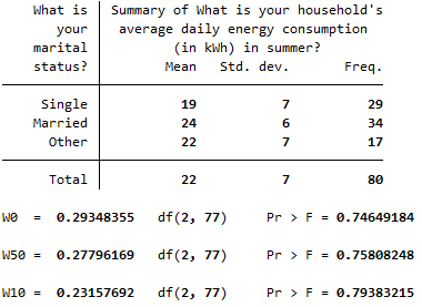
The \(p\) value for Levene’s Test for Equality of Variances (listed in the first row below the table, after \(Pr > F =\)) is \(p > .05\) (in fact \(p = .746\)), so we can assume equal variances in this case. If the equal variances assumption is violated you will need to use a Welch or Brown-Forsythe statistic instead.
-
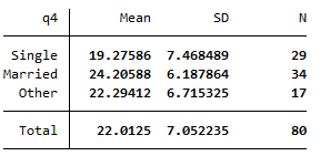
If all the assumptions are met you can conduct the one-way ANOVA in Stata. You can do this using the anova command, which you may like to combine with the tabstat command (to obtain a table of descriptive statistics as part of the output) as follows:
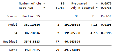
tabstat q6, by(q4) stats (mean sd n)
anova q6 q4
The output should look like this:
-
From the descriptive statistics table we can see that the mean summer daily energy consumption in our sample for those who are single is \(19.28\)kWh, for those who are married it is \(24.21\)kWh and for those who classified their marital status as ‘Other’ it is \(22.29\)kWh. To test whether there are any statistically significant differences between these values, we need to refer to the ANOVA table and to the \(p\) value. Since \(p < .05\) (in fact \(p = .0195\)) we can reject the null hypothesis and conclude that the mean summer daily energy consumption is significantly different for at least one of the marital status groups.
To find out where the significant difference(s) lie you can conduct a post hoc test. While there are many different options to choose from, a common test to try is Tukey’s HSD test. To obtain output for this you can run the pwcompare command as follows:
pwcompare q4, mcompare(tukey)The output should be as shown:
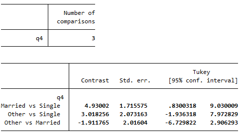
From this table we can observe that the only significant difference in mean summer daily energy consumption is between the married and single groups. This is shown by the fact that the confidence interval for the difference in mean energy consumption between married and single people is the only confidence interval that does not contain the null value of zero.