Introduction to SPSS

Often when you are doing your analysis you will find that it is helpful to create new variables, or to make changes to existing variables. This page details some of the transformation facilities provided by SPSS which enable you to do this, all of which are found under the Transform menu.

Note that the examples covered here make use of the Household energy consumption data.sav file, which contains fictitious data for 80 people based on a short ‘Household energy consumption’ questionnaire. If you want to work through the examples provided you can download the data file using the following link:

• Household energy consumption data [SAV, 8kB]

If you would like to read the sample questionnaire for which the data relates, you can do so using this link:

• Household energy consumption questionnaire [PDF, 187kB]

Before commencing the analysis, note that the default is for dialog boxes in SPSS to display any variable labels, rather than variable names. You may find this helpful, but if you would prefer to view the variable names instead then from the menu choose:

• Edit
• Options…
• Change the Variable Lists option to Display names

Computing a new variable

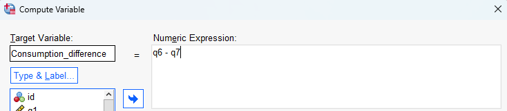
Sometimes you may wish to create a new variable or variables to add to your data file, either from scratch or using the data from an existing variable or variables. For example, in the sample data file you may wish to create a new variable which gives the difference between summer and winter household energy consumption for each survey participant. You can do this by choosing the following from the SPSS menu (either from the Data Editor or Output window):

• Transform
• Compute Variable…
• specify the new variable name in the Target Variable box, for example ‘Consumption_difference’
• enter the required formula in the Numeric Expression box, for example by moving the ‘q6’ variable into the box, using the keypad provided or your keyboard to type the - (minus) sign, and then moving the ‘q7’ variable into the box (spaces between each item are optional)

Next:

• click OK

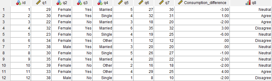
If you then navigate to the Data View of the Data Editor window, you will see that a new ‘Consumption_difference’ variable has been added to the end of the data file, with the difference for each of the 80 cases determined using the numeric expression entered. You can then analyse this variable as you would any of the original variables.

Note that you can also move the new variable if wished, either in the Data View or in the Variable View, by dragging and dropping. For example, you could move the new variable to sit after the ‘q7’ variable by selecting the variable name in the Data View, then holding down the left mouse key and dragging until it is in the required spot.

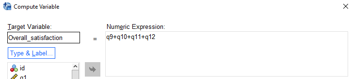
As another example of when you might want to compute a new variable, consider questions q9 through q12, which all relate to satisfaction with different aspects of the participants’ electricity provider. As these questions all use the same rating system (measured on a scale of 1 to 5, with 1 indicating ‘Very unsatisfied’ and 5 indicating ‘Very satisfied’), the four variables representing these questions can be combined to come up with an overall satisfaction score.

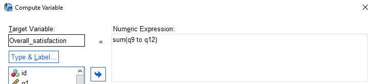
One way of doing this is by adding all the variables together to create a score out of 20. To do this, you could enter the new variable name Overall_satisfaction and the numeric expression q9+q10+q11+q12:

If you run the Frequencies procedure on this new variable (as described in the Descriptive statistics page of this module) you will see that there are only 78 satisfaction scores, whereas there are 80 cases in the data file. Looking at the actual data reveals why; the data in row 30 is missing for all four of the variables ‘q9’ to ‘q12’, and the data in row 31 is missing for variables ‘q10’ and ‘q12’. Since the numeric expression shown above only calculates new values for those cases that have complete data, the new variable has not been computed for rows 30 and 31.

Sometimes this will be what you want, but other times you will require data for the new variable regardless of whether some of the data is missing or not (note that if there is missing data for all the variables, there will automatically be missing data for the new variable). To do this simply requires that a different numeric expression is used within the Compute variable procedure, which makes use of the sum function.

For example, you could alter the numeric expression for the variable you have just created to sum(q9 to q12) (note that the word ‘to’ can be used between the variables in this case as they occur one after the other in the data file; if this isn’t the case, you would need to list the variable names separated by commas instead):

With this new numeric expression, there is now a value for the ‘Overall_satisfaction’ variable in row 31.

You may also like to experiment with other formulas. For example, if you wanted to calculate an average overall satisfaction score instead you could also try using two different, similar numeric expressions:

• The numeric expression (q9 + q10+ q11 + q12)/4 will again have missing data for both rows 30 and 31.
• The numeric expression mean(q9 to q12) (or mean(q9, q10, q11, q12) if the variables are not in order) will have missing data only for row 30. For row 31, the average will be calculated by dividing by 2 instead of 4, since there are only two variables with data.

Regardless of which formula you choose to use, the new variable can then be analysed in the usual way.

Recoding an existing variable

Sometimes you may wish to recode an existing categorical variable, most likely to reduce the number of categories by combining existing ones together. For example, in the sample data file you may wish to recode the ‘q8’ variable to reduce the number of categories from five to three. You can do this by choosing the following from the SPSS menu (either from the Data Editor or Output window):

• Transform
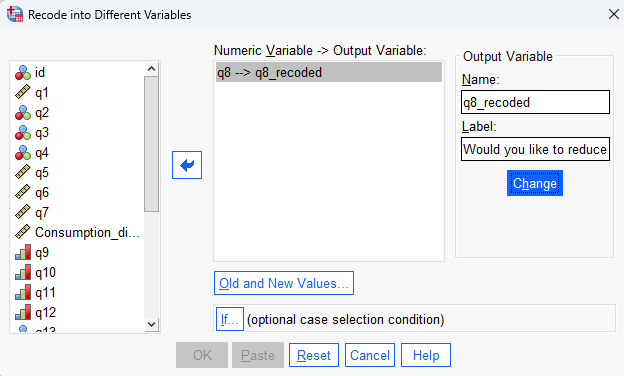
• Recode into Different Variables… (this will keep the existing variable and create a new one, which provides maximum flexibility; if you would prefer to over-write the existing variable though you can select Recode into Same Variables…)
• move the required variable into the Numeric Variable - > Output Variable box, for example ‘q8’
• specify a name for the new variable in the Name field of the Output Variable box, for example ‘q8_recoded’
• enter a label for the new variable in the Label field of the Output Variable box if desired
• click Change

The second part of the process is to decide how the categories of the existing variable are going to map to categories of the new variable. Sometimes this can require quite a bit of thought and planning, but with so few categories in this example it is more straightforward. In particular, the existing categories lend themselves to being recoded into three new categories (‘Agree’, ‘Neutral’ and ‘Disagree’), as follows:

Existing category	New category
1 (Strongly disagree)	1 (Disagree)
2 (Disagree)	1 (Disagree)
3 (Neutral)	2 (Neutral)
4 (Agree)	3 (Agree)
5 (Strongly agree)	3 (Agree)

To specify this in SPSS, do the following in the Recode into Different Variables: Old and New Values dialogue box:

• select Old and New Values…
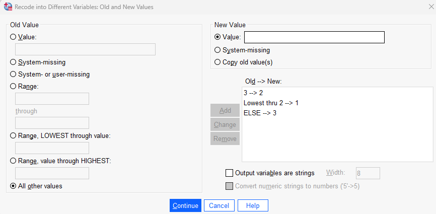
• specify the existing category number(s) in the Old Value side of the dialogue box, and the new category number in the New Value side of the dialogue box, then press Add. You can map each category individually, or multiple categories can be mapped at once using the options available. For example, you could specify the required mappings as follows:
• select Range, LOWEST through value: and specify 2 on the Old Value side of the dialogue box, and specify 1 on the New Value side of the dialogue box, then press Add
• select Value: and specify 3 on the Old Value side of the dialogue box, and specify 2 on the New Value side of the dialogue box, then press Add
• select All other values and specify 3 on the New Value side of the dialogue box, then press Add
• click Continue

Next:

• click OK

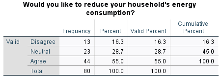
If you then navigate to the Data View of the Data Editor window, you will see that a new ‘q8_recoded’ variable has been added to the end of the data file (note that you can move it if wished, either in the Data View or in the Variable View, by dragging and dropping). The category values do not currently have any labels (e.g. ‘Disagree’, ‘Neutral’ and ‘Agree’), and you may need to change the variable Measure (from Nominal to Ordinal), but you can do both of these things as described in the Getting started page of this module.

Once you have finished setting up the variable, you can analyse it in the usual way. For example, you could run the Frequencies procedure (as described in the Descriptive statistics page of this module) on the new variable, which should result in the following table:

Converting a string variable

Although SPSS does allow alphabetic/string information to be entered as part of the data file, the more in-depth statistical analysis procedures require numeric data only (even if those numbers are simply codes or values representing categories).

At the questionnaire design stage it may be very difficult to anticipate the responses that will be given though, so creating a tick-box type question can be too complicated or restrictive. Hence allowing open-ended responses may be preferable instead, and the choice then is to either numerically code the data before keying it in, or to recode the responses once they have been entered into SPSS. This section details how to do the latter using the Automatic Recode and Recode into Different/Same Variable procedures, and uses the ‘q13’ variable in the sample data file as an example. This variable stores participant responses to the question:

What kind of hot water system do you use at your property?

The variable is defined as String under Variable View, and is a nominal variable. A frequency table of the responses is as follows:

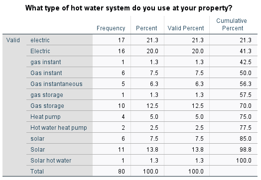
This output shows only five different types of hot water systems, but because of different spelling and terminology and different use of upper and lower case characters, twelve different responses are listed. To reduce this twelve down to the real five, the different categories need to be combined (i.e. recoded).

To complete the first part of this two-step process, from the menus choose:

• Transform
• Automatic Recode…

Now in the dialogue box that opens:

• move the variable (‘q13’) into the Variables box
• enter a name for the new variable in the New Name box (for example ‘q13_autorecode’)
• click on Add New Name
• select Treat blank string variables as user-missing (so that no category is created for these)
• select OK

The resultant output should be as follows:

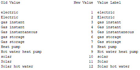
Note that the original responses have been sorted into alphabetical order and assigned a value from 1 to 12. The original data has been used to create the Value Labels for those values and all this has been put into a new variable at the end of the data file called ‘q13_autorecode’.

The second step of the process is then to reduce these 12 categories to the 5 required ones, using the standard Recode into Different Variables command described previously (or you could use the Recode into Same Variables command in this instance if preferred). In this case, the existing and new categories could be as follows:

Existing category	New category
1 (electric)	1 (Electric)
2 (electric)	1 (Electric)
3 (gas instant)	2 (Instantaneous gas)
4 (Gas instant)	2 (Instantaneous gas)
5 (Gas instantaneous)	2 (Instantaneous gas)
6 (gas storage)	3 (Gas storage)
7 (Gas storage)	3 (Gas storage)
8 (Heat pump)	4 (Heat pump)
9 (Hot water heat pump)	4 (Heat pump)
10 (solar)	5 (Solar)
11 (Solar)	5 (Solar)
12 (Solar hot water)	5 (Solar)

Visual binning

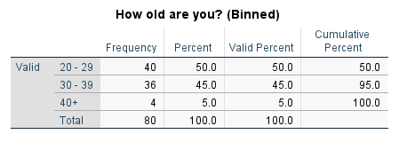
Sometimes it is helpful to transform a continuous variable into a categorical variable, as this provides additional analysis options. For example, in the sample data file you may wish to transform the continuous ‘q1’ variable into categories, perhaps in order to make some comparisons for different age groups.

While you can in fact do this using either of the procedures outlined above, the purpose-built procedure for this in SPSS is Visual Binning. You can make use of this by choosing the following from the SPSS menu (either from the Data Editor or Output window):

• Transform
• Visual Binning…
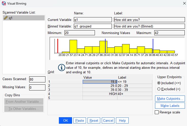
• select the required variable, for example the ‘q1’ variable, and move it across to the Variables to Bin box
• select Continue
• specify a name for the new variable in the Binned Variable box, for example ‘q1_grouped’
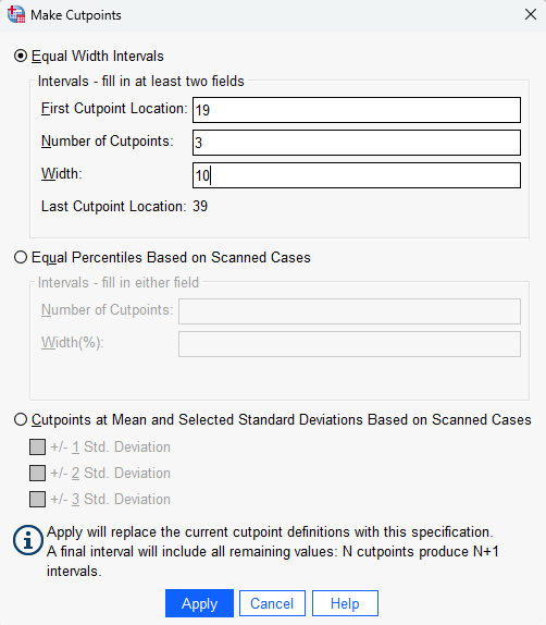
• click on the Make Cutpoints… button, to specify how you are going to ‘cut’ the data in order to make categories (sometimes you might use the histogram of the data to help you decide how to do this, while other times you might have set categories already in mind)
• specify a value for the First Cutpoint Location, for example if you want the first age category to include those up to and including the age of 19, you would enter 19
• specify the Number of Cutpoints , which will be one less than the number of categories you want to have, for example if you want to have four age categories you would enter 3
• adjust the Width of each cutpoint, for example from 7.667 to 10

Next:

• click Apply
• click Make Labels to automatically create labels for each new category

Next:

• click OK

If you then navigate to the Data View of the Data Editor window, you will see that a new ‘q1_grouped’ variable has been added to the end of the data file (note that you can move it if wished, either in the Data View or in the Variable View , by dragging and dropping). You can analyse it in the usual way, for example you could run the Frequencies procedure (as described in the Descriptive statistics page of this module) on the new variable, which should result in the following table: