Data literacy with R
Real World Datasets
There are many sources of data on the internet. Governments make public sector data available for activities such as Hackathons, allowing diverse groups of people to provide innovative solutions for communities.
For example, the West Australian State Government has the site Data WA, with over 2000 datasets.
The Australian Government has the site data.gov.au, with over 100,000 datasets.
Another good source is the Australian Bureau of Statistics (ABS)
Dataset 1 - Accessing and Cleaning
Our first dataset is Australian Taxation Statistics 2021-2022, in particular Table 6B which gives summary tax details for individual returns by postcode.
This dataset can be accessed directly from R, it is an Excel xlsx file. It is published under a Creative Commons Attribution 2.5 Australia licence so is suitable for use here.
Previewing this file, the data really starts in row 2 with the column names. Let’s say we are only interested in some data, somewhat arbitrarily Taxable Income and Private Health cover status related data across States and Postcodes. So we only need to import Columns 1, 3, 4, 6 and 155.
tax2022_url <- 'https://data.gov.au/data/dataset/4be150cc-8f84-46b8-8c61-55ff1d48a700/resource/43d41d1d-4e39-45df-b693-a06255779cff/download/ts22individual06taxablestatusstatesa4postcode.xlsx'

download.file(tax2022_url, 'tax2022.xlsx', mode = 'wb')

tax2022_raw <- read_excel('tax2022.xlsx', sheet = 'Table 6B', skip = 1, col_names = TRUE)[ ,c(1,3,4,6,155)]

tax2022_raw$Postcode <- str_pad(tax2022_raw$Postcode, 4, side="left", pad="0")

head(tax2022_raw, 5)
| State/ Territory1 | Postcode | Individuals no. | Taxable income or loss4 $ | People with private health insurance no. |
|---|---|---|---|---|
| <chr> | <chr> | <dbl> | <dbl> | <dbl> |
| ACT | 2600 | 5951 | 791214764 | 4841 |
| ACT | 2601 | 3614 | 265604097 | 1965 |
| ACT | 2602 | 23085 | 2026942835 | 15791 |
| ACT | 2603 | 7558 | 1055186744 | 5926 |
| ACT | 2604 | 9137 | 953261746 | 6649 |
R provides the functionality to change the column names to something easier to work with.
names(tax2022_raw) <- c('State', 'Postcode', 'Returns', 'TaxableIncome_dollars', 'PrivateHealth_returns')
head(tax2022_raw)
| State | Postcode | Returns | TaxableIncome_dollars | PrivateHealth_returns |
|---|---|---|---|---|
| <chr> | <chr> | <dbl> | <dbl> | <dbl> |
| ACT | 2600 | 5951 | 791214764 | 4841 |
| ACT | 2601 | 3614 | 265604097 | 1965 |
| ACT | 2602 | 23085 | 2026942835 | 15791 |
| ACT | 2603 | 7558 | 1055186744 | 5926 |
| ACT | 2604 | 9137 | 953261746 | 6649 |
| ACT | 2605 | 8111 | 863964219 | 6298 |
Using only code, R provides the ability to look at the structure (str()) and summary (sum()) of the data.
- Structure
str(tax2022_raw)
tibble [2,639 × 5] (S3: tbl_df/tbl/data.frame)
 $ State                : chr [1:2639] "ACT" "ACT" "ACT" "ACT" ...
 $ Postcode             : chr [1:2639] "2600" "2601" "2602" "2603" ...
 $ Returns              : num [1:2639] 5951 3614 23085 7558 9137 ...
 $ TaxableIncome_dollars: num [1:2639] 7.91e+08 2.66e+08 2.03e+09 1.06e+09 9.53e+08 ...
 $ PrivateHealth_returns: num [1:2639] 4841 1965 15791 5926 6649 ...
- Summary
summary(tax2022_raw)
    State             Postcode            Returns         TaxableIncome_dollars
 Length:2639        Length:2639        Min.   :    51.0   Min.   :1.368e+06
 Class :character   Class :character   1st Qu.:   412.5   1st Qu.:2.389e+07
 Mode  :character   Mode  :character   Median :  2103.0   Median :1.300e+08
                                       Mean   :  5886.9   Mean   :4.258e+08
                                       3rd Qu.:  8608.5   3rd Qu.:6.247e+08
                                       Max.   :123657.0   Max.   :5.074e+09
 PrivateHealth_returns
 Min.   :   12
 1st Qu.:  212
 Median : 1079
 Mean   : 3312
 3rd Qu.: 5010
 Max.   :36635
To filter rows, columns, or any combination of these, there are multiple ways of achieving this in R. R uses 1-based indexing, the first index of a list is 1.
Filter by
- Columns/Fields, either by column number
head(tax2022_raw[ , 2], 3) # 2nd column
| Postcode |
|---|
| <chr> |
| 2600 |
| 2601 |
| 2602 |
- or by Column ‘Name’,
head(tax2022_raw[ , "Postcode"], 4)
| Postcode |
|---|
| <chr> |
| 2600 |
| 2601 |
| 2602 |
| 2603 |
- or alternatively (with tail instead of head, to access the last rows of the data frame),
tail(tax2022_raw$Postcode, 4)
- '6951'
- '6959'
- '6985'
- 'WA other'
- to retrieve the unique values from a column,
unique(tax2022_raw$State)
- 'ACT'
- 'NSW'
- 'NT'
- 'Overseas'
- 'QLD'
- 'SA'
- 'TAS'
- 'VIC'
- 'WA'
- Rows/Records, either by row number,
tax2022_raw[2, ]
| State | Postcode | Returns | TaxableIncome_dollars | PrivateHealth_returns |
|---|---|---|---|---|
| <chr> | <chr> | <dbl> | <dbl> | <dbl> |
| ACT | 2601 | 3614 | 265604097 | 1965 |
- by rows which have particular values (or categories) in a column,
tax2022_raw[tax2022_raw$State %in% c("Unknown","Overseas"),]
| State | Postcode | Returns | TaxableIncome_dollars | PrivateHealth_returns |
|---|---|---|---|---|
| <chr> | <chr> | <dbl> | <dbl> | <dbl> |
| Overseas | Overseas | 123657 | 3888397917 | 17557 |
- by Rows and Columns, either by row and column number,
tax2022_raw[2,2]
| Postcode |
|---|
| <chr> |
| 2601 |
- or by the row with the maximum value of a column, and returning only three columns of the dataframe.
tax2022_raw[tax2022_raw$PrivateHealth_returns == max(tax2022_raw$PrivateHealth_returns), c(1,2,5)]
| State | Postcode | PrivateHealth_returns |
|---|---|---|
| <chr> | <chr> | <dbl> |
| QLD | 4350 | 36635 |
There are two interesting aspects of the data above which demonstrate the need to ‘clean’ data.
-
The tail command above reveals that the data is not exclusively ‘per postcode’; if the number of returns was small those postcodes are grouped into an ‘Other’ row. We will leave this for the moment and observe the impact later in this workflow.
-
There are some State values of ‘Overseas’ or ‘Unknown’ which are not of interest. In base R we would create a new dataframe without these. We can also check the new dataframe with the filter to check that it returns no matching rows.
# Create an new, intermediate table without these rows
tax2022_raw_aus <- tax2022_raw[!(tax2022_raw$State %in% c("Unknown","Overseas")),]

# Check the rows are now excluded
str(tax2022_raw_aus[tax2022_raw_aus$State %in% c("Unknown","Overseas"),])
tibble [0 × 5] (S3: tbl_df/tbl/data.frame)
 $ State                : chr(0)
 $ Postcode             : chr(0)
 $ Returns              : num(0)
 $ TaxableIncome_dollars: num(0)
 $ PrivateHealth_returns: num(0)
The Tidyverse!
In cleaning and subsetting the data above we now have two data frames, namely tax2022_raw and tax2022_raw_aus. In trying to keep the R commands relatively short and understandable we can end up with a lot of intermediate or temporary data frames, which can be difficult to keep track of. We could choose to not create the intermediate dataframes using a lot of ‘nesting’, though this leads to long complicated commands with lots of brackets! Another alternative is to use pipes, where the output of one command is ‘piped’ into the next command and so on. This strikes a great balance between command readability and minimising intermediate data frames.
There is an R package called Tidyverse, which includes a set of key R extension packages (including dplyr and tidyr) intended to make using (and learning) R easier for beginners. It includes the piping functionality, along with functions which filter, reshape and plot data. We will use the Tidyverse commands in the following analysis. In fact we already have, using read_excel above.
For example, to achieve removing the same rows in the previous step, we can ‘pipe’ the tax2022_raw data to the filter() command from the Tidyverse and compare the total rows with the previous str() command. The symbol for pipe is %>%, the keyboard shortcut for which is Ctrl+Shift+M, or Command+Shift+M on a Mac, when working in R or RStudio (once again not in our Jupyter Notebooks).
Note that the str() command, as do many commands, plays nicely with the piping too.
tax2022_raw %>%
  filter( State !="Unknown" & State!="Overseas" ) %>%
  str()
tibble [2,638 × 5] (S3: tbl_df/tbl/data.frame)
 $ State                : chr [1:2638] "ACT" "ACT" "ACT" "ACT" ...
 $ Postcode             : chr [1:2638] "2600" "2601" "2602" "2603" ...
 $ Returns              : num [1:2638] 5951 3614 23085 7558 9137 ...
 $ TaxableIncome_dollars: num [1:2638] 7.91e+08 2.66e+08 2.03e+09 1.06e+09 9.53e+08 ...
 $ PrivateHealth_returns: num [1:2638] 4841 1965 15791 5926 6649 ...
Key Learning
Key Learning #1 - Data is data, there is no need to constantly have a dedicated view for the raw, original data. These tools allow us to view it in any form needed so as to inform our analysis and visualisation.
Key Learning #2 - Cleaning the data involves investigating the original data, leaving it as it is and writing code to create a workable dataset, having removed unnecessary or incorrect data.
Key Learning #3 - Using pipes makes it simpler to prepare, read and modify code and eliminates the need for the clutter of many intermediate or temporary data frames.
Further Learning
Further Learning #1 - The datasets in this workshop are quite ‘clean’ and complete. Then there are datasets which are incomplete with data that is not available or NA - for another time.
Dataset 1 - Analysis
As an example, let’s perform some aggregate functions, such as sums or totals of dollars and returns for each State. Whereas filter() acts on rows, select() acts on columns. We will aggregate by State, so we remove the Postcode column using select(). We could select the rows we require as per above, however here it is more convenient to drop the few column(s) we don’t require. The !Postcode here is read as ‘select all columns that are not the Postcode column’.
To calculate the sums we can pipe the data to a group_by() command to group by State, and then pipe that result to a summarise_all() command to perform the aggregation on all columns. It’s also possible to use summarise() to sum individual columns.
# Totals by State
tax2022_raw %>%
  filter( State !="Unknown" & State!="Overseas" ) %>%
  select(!Postcode) %>%
  group_by(State) %>%
  summarise_all(sum)
| State | Returns | TaxableIncome_dollars | PrivateHealth_returns |
|---|---|---|---|
| <chr> | <dbl> | <dbl> | <dbl> |
| ACT | 301650 | 25305959656 | 199369 |
| NSW | 4788259 | 366314190746 | 2832812 |
| NT | 132529 | 9640785020 | 66821 |
| QLD | 3156186 | 216127627636 | 1607801 |
| SA | 1065717 | 68138353958 | 638572 |
| TAS | 329221 | 20005188929 | 171046 |
| VIC | 3958298 | 284549647726 | 2054944 |
| WA | 1679878 | 129655460938 | 1151554 |
To calculate the sums for the whole of Australia for 2019-2020, let’s filter the State column too.
# Totals for Australia
tax2022_raw %>%
  filter( State !="Unknown" & State!="Overseas" ) %>%
  select(!c('Postcode', 'State')) %>%
  summarise_all(sum)
| Returns | TaxableIncome_dollars | PrivateHealth_returns |
|---|---|---|
| <dbl> | <dbl> | <dbl> |
| 15411738 | 1.119737e+12 | 8722919 |
As a further example, let’s calculate the
- Taxable Income per return per State, and
- Percent of Private Health Insurance per State
Here we are creating two new calculated columns based on the data for each row, and so will use the mutate() command to create the new columns and mean for the summary.
# Means per State
tax2022_raw %>%
  filter( State !="Unknown" & State!="Overseas" ) %>%
  mutate(TaxableIncome_dollarspr = TaxableIncome_dollars/Returns) %>%
  mutate(PrivateHealth_percentpp = PrivateHealth_returns/Returns*100) %>%
  select(State, TaxableIncome_dollarspr, PrivateHealth_percentpp ) %>%
  group_by(State) %>%
  summarise_all(mean)
| State | TaxableIncome_dollarspr | PrivateHealth_percentpp |
|---|---|---|
| <chr> | <dbl> | <dbl> |
| ACT | 86592.31 | 64.49100 |
| NSW | 71809.85 | 60.11323 |
| NT | 72862.82 | 49.59776 |
| QLD | 63037.80 | 50.04635 |
| SA | 60967.22 | 58.45886 |
| TAS | 58154.11 | 50.85241 |
| VIC | 66824.78 | 49.70195 |
| WA | 73781.56 | 66.53637 |
Wide and Narrow Formats
The raw data is in summary form, or wide form. Easily read by people, not ideal for all the processing options available for machines eg AI.
Sometimes tasks in R are more easily achieved with the data in narrow or long format, where each row essentially only has one item of data.
Fortunately R and the tidyverse have tools which allow for easily swapping between formats, namely pivot_wider and pivot_longer.
What is important is knowing which columns are to be kept, often called identifier variables ( Postcode and State ), and which columns are to be pivoted, often called measured variables ( Returns, Taxable Income and Private Health status ).
Let’s create a temporary dataframe tax2022_raw_long here just to show the effect of moving from wide to narrow/long formats and back again.
From Wide to Narrow/Long
tax2022_raw_long <- tax2022_raw %>%
  filter( State !="Unknown" & State!="Overseas" ) %>%
  pivot_longer( cols = -c(Postcode, State),
                names_to = "item",
                values_to = "value",
                values_drop_na = TRUE)
head(tax2022_raw_long)
| State | Postcode | item | value |
|---|---|---|---|
| <chr> | <chr> | <chr> | <dbl> |
| ACT | 2600 | Returns | 5951 |
| ACT | 2600 | TaxableIncome_dollars | 791214764 |
| ACT | 2600 | PrivateHealth_returns | 4841 |
| ACT | 2601 | Returns | 3614 |
| ACT | 2601 | TaxableIncome_dollars | 265604097 |
| ACT | 2601 | PrivateHealth_returns | 1965 |
and then back from Narrow/Long to Wide
tax2022_raw_long %>%
  pivot_wider( names_from = "item",
               values_from = "value") %>%
  head()
| State | Postcode | Returns | TaxableIncome_dollars | PrivateHealth_returns |
|---|---|---|---|---|
| <chr> | <chr> | <dbl> | <dbl> | <dbl> |
| ACT | 2600 | 5951 | 791214764 | 4841 |
| ACT | 2601 | 3614 | 265604097 | 1965 |
| ACT | 2602 | 23085 | 2026942835 | 15791 |
| ACT | 2603 | 7558 | 1055186744 | 5926 |
| ACT | 2604 | 9137 | 953261746 | 6649 |
| ACT | 2605 | 8111 | 863964219 | 6298 |
Visualisation and ggplot
R also has functions to visualise data. One common library used for visualisations is ggplot2, which is included in the tidyverse.
The code defines the data to be used, and then we use code to generate the graphs and assign values to the different aspects of the graphs. Code generated visualisation can be very efficient compared to GUI based platforms.
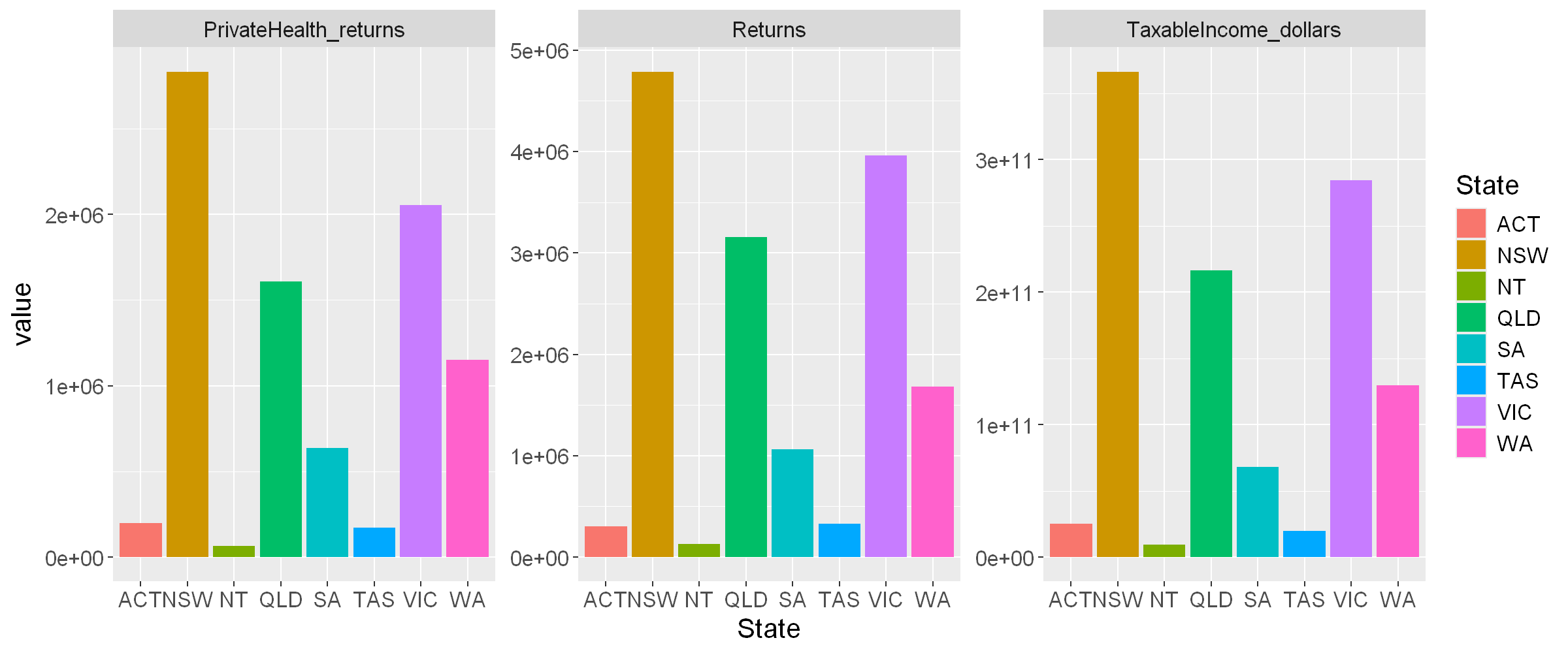
For example, to quickly visualise (without much styling!) the summed totals of the raw data per State
- we take the code from earlier (#Totals by State),
- use pivot_longer() to transform from wide to narrow/long format ready for ggplot, keeping the State as the identifier column,
- use ggplot(), adding geom_bar() for the bargraph and a facet_wrap() to show the different items in separate facets, each with independent y axis ranges (thanks to ‘free_y’ scaling)
Note that here we need to assign the output of ggplot to a variable plot_states using <- and then display the contents of that variable, which is the plot.
plot2022_states_totals <- tax2022_raw %>%
  filter( State !="Unknown" & State!="Overseas" ) %>%
  select(!Postcode) %>%
  group_by(State) %>%
  summarise_all(sum) %>%
  pivot_longer( cols = -c(State),
                names_to = "item",
                values_to = "value",
                values_drop_na = TRUE) %>%
  ggplot(aes(x=State, y=value, fill=State)) +
  geom_bar(stat = "identity") + facet_wrap( vars(item), scales="free_y") +
  theme(text = element_text(size = 15))

plot2022_states_totals
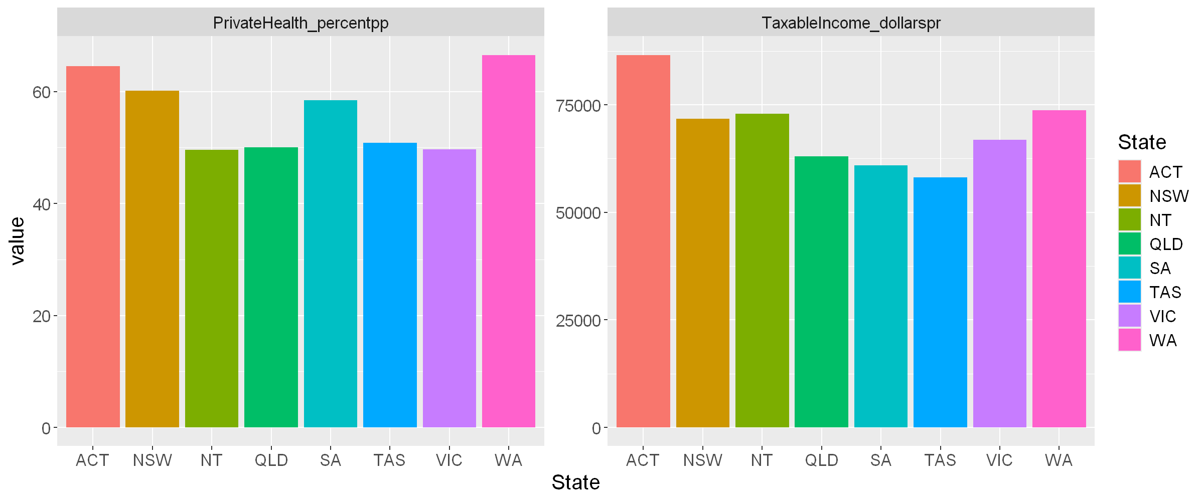
To quickly visualise the mean values per state
- we take the code from earlier (#Means per State),
- use pivot_longer() and ggplot() as before to produce the graph.
plot2022_state_means <- tax2022_raw %>%
  filter( State !="Unknown" & State!="Overseas" ) %>%
  mutate(TaxableIncome_dollarspr = TaxableIncome_dollars/Returns) %>%
  mutate(PrivateHealth_percentpp = PrivateHealth_returns/Returns*100) %>%
  select(State, TaxableIncome_dollarspr, PrivateHealth_percentpp ) %>%
  group_by(State) %>%
  summarise_all(mean) %>%
  pivot_longer( cols = -c(State),
                names_to = "item",
                values_to = "value",
                values_drop_na = TRUE) %>%
  ggplot(aes(x=State, y=value, fill=State)) +
  geom_bar(stat = "identity") + facet_wrap( vars(item), scales="free_y") +
  theme(text = element_text(size = 15))

plot2022_state_means
Note: These plots are images; they can become blurry when enlarged and are not responsive on different devices such as mobiles or tablets. Other visualisation tools, such as Leaflet and Plotly (presented later) are more versatile as they effectively recreate the plot to suit each device.
Automation
When the source data changes, for example more data samples are collected or updated, using code to manipulate the data brings a massive advantage - automation. The same code can be re-executed on the new data for updated analysis and visualisations.
As an example, here is the code used to sum the three Taxation parameters for Australia for 2021-2022, re-executed for the 2020-2021 dataset, also published under Creative Commons Attribution 2.5 Australia. The code required a small tweak, the columns are in a different order compared to 2021-2022.
Compare the results for 2020/21 and 2021/22.
- 2020/2021
tax2021_url <- 'https://data.gov.au/data/dataset/07b51b39-254a-4177-8b4c-497f17eddb80/resource/fa05bac8-079d-4eba-bd4d-779466e45f02/download/ts21individual06taxablestatusstateterritorypostcode.xlsx'

download.file(tax2021_url, 'tax2021.xlsx', mode = 'wb')

tax2021_raw <- read_excel('tax2021.xlsx', sheet = 'Table 6B', skip = 1, col_names = TRUE)[ ,c(1,2,3,5,154)]

names(tax2021_raw) <- c('State', 'Postcode', 'Returns', 'TaxableIncome_dollars', 'PrivateHealth_returns')

tax2021_raw %>%
  filter( State !="Unknown" & State!="Overseas" ) %>%
  mutate(TaxableIncome_dollarspr = TaxableIncome_dollars/Returns) %>%
  mutate(PrivateHealth_percentpp = PrivateHealth_returns/Returns*100) %>%
  select(TaxableIncome_dollarspr, PrivateHealth_percentpp ) %>%
  summarise_all(mean)
| TaxableIncome_dollarspr | PrivateHealth_percentpp |
|---|---|
| <dbl> | <dbl> |
| 62881.6 | 55.71372 |
- 2021/22
tax2022_raw %>%
  filter( State !="Unknown" & State!="Overseas" ) %>%
  mutate(TaxableIncome_dollarspr = TaxableIncome_dollars/Returns) %>%
  mutate(PrivateHealth_percentpp = PrivateHealth_returns/Returns*100) %>%
  select(TaxableIncome_dollarspr, PrivateHealth_percentpp ) %>%
  summarise_all(mean)
| TaxableIncome_dollarspr | PrivateHealth_percentpp |
|---|---|
| <dbl> | <dbl> |
| 67519.74 | 55.81243 |
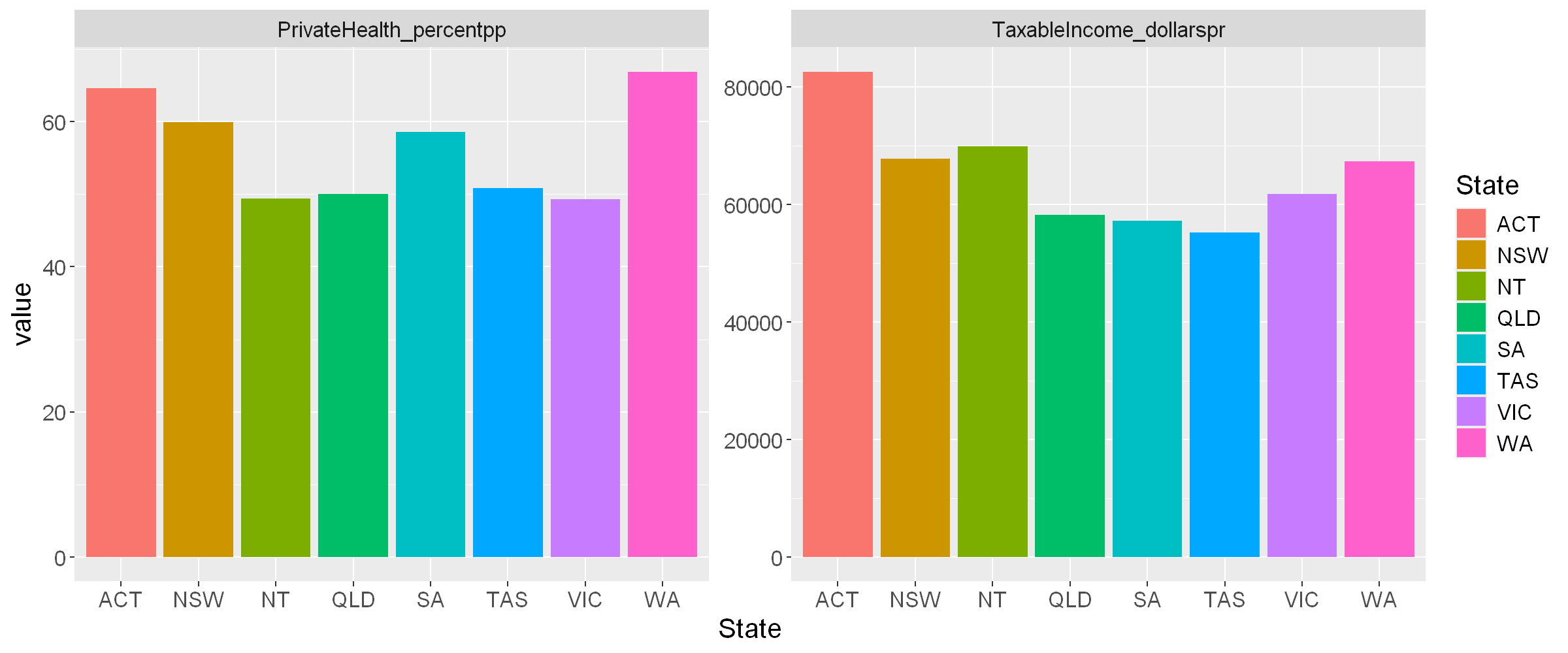
Also compare the plot of mean values for 2020/21.
plot2021_state_means <- tax2021_raw %>%
  filter( State !="Unknown" & State!="Overseas" ) %>%
  mutate(TaxableIncome_dollarspr = TaxableIncome_dollars/Returns) %>%
  mutate(PrivateHealth_percentpp = PrivateHealth_returns/Returns*100) %>%
  select(State, TaxableIncome_dollarspr, PrivateHealth_percentpp ) %>%
  group_by(State) %>%
  summarise_all(mean) %>%
  pivot_longer( cols = -c(State),
                names_to = "item",
                values_to = "value",
                values_drop_na = TRUE) %>%
  ggplot(aes(x=State, y=value, fill=State)) +
  geom_bar(stat = "identity") + facet_wrap( vars(item), scales="free_y") +
  theme(text = element_text(size = 15))

plot2021_state_means
Key Learning
Key Learning #4 - Data frame structures are easily transformed in R, transforming to whatever form is convenient for a particular purpose.
Key Learning #5 - Using code to perform analysis and generate graphs and visualisations saves a lot of time and finessing, particularly when tasks need to be repeated regularly and often.
Further Learning
Further Learning #2 - The above visualisations were generated quickly, without too much concern for formatting. Every aspect of the graphs above can be controlled to give beautiful and purposeful visualisations.