
Introduction-to-statistics-printable-guide-UniSkills.pdf
Introduction to statistics
Table of Contents
Introduction
Welcome to the Introduction to statistics module. This module introduces key ideas that will help you understand statistics used in journal articles and other academic literature, and that you can use to analyse your own data. Note that if you are not planning to do either of these things, and instead only want to learn how to interpret a small number of common graphs and tables and calculate a few important values, you may find the Statistics and probability page of the Numeracy fundamentals module more suitable.
You can work through this module from beginning to end in the order provided, or you can move directly to specific pages or sections based on your needs or preferences. Additionally, if you are interested in learning how to carry out the statistical tests discussed in this module using the statistical software SPSS or Stata, you may also wish to complete the Introduction to SPSS or Introduction to Stata module. Note that all graphs and tables included in this module have been created using SPSS, except the tables in the Interpreting statistics page which have been taken from journal articles.
Before starting the module, you may also find it helpful to read the How to get confident with statistics post on The Research Whisperer blog. This post provides practical advice on building confidence in statistics and may help you make better use of this module.
Your feedback on this module is welcome at any time and can be provided through the feedback page. If you have questions about the module, please contact Library-UniSkills@curtin.edu.au
What you will learn
- What data and variables are, and how to identify different types, including categorical and continuous data and independent and dependent variables.
- How to interpret and critically evaluate statistics published in academic sources, including how to tell the difference between descriptive and inferential statistics and between statistical and practical significance.
- What descriptive statistics are, and how to display data and calculate descriptive statistics for one variable or two variables at a time, for both categorical and continuous data.
- What the normal distribution and sampling distributions are, and how to determine whether a variable is normally distributed or whether a sample size is large enough for the sampling distribution of the mean to be treated as a normal distribution.
- What inferential statistics are, including how to distinguish between estimation and hypothesis testing, how to calculate confidence intervals, and how to interpret confidence intervals and \(p\) values.
- How to compare the means of continuous variables using \(t\)-tests or one-way analysis of variance (ANOVA).
- How to test for relationships between pairs of variables using the chi-square test of independence or Pearson’s correlation.
- How to use linear and logistic regression to understand and explain relationships between variables.Data & variable types
This page details some important concepts that will be referred to in subsequent pages, including what data and variables are, and how to distinguish between different types.
In brief, it covers the following:
- A definition of data
- A definition of a variable
- How to distinguish between categorical and continuous data
- How to distinguish between independent and dependent variables
</div>
What is data?
The word data refers to observations and measurements which have been collected in some way, often through research.
Data that is recorded as numbers (and therefore measures quantities) is quantitative data, while data that is recorded as text (and therefore records qualities) is qualitative data. Quantitative data can be analysed using statistics, as can qualitative data that records qualities in terms of different categories (for example what hair colour someone has, what country someone was born in, what their marital status is, etc.), as opposed to data that records qualities in terms of thoughts, feelings and opinions.
It is the former two types of data that you will be working with in this module, and shortly we will introduce some other terms that are typically used in statistics to describe data of this nature.
What is a variable?
Variables are the characteristics or attributes that you are observing, measuring and recording data for. Some examples include height, weight, eye colour, dog breed, climate, electrical conductivity, customer service satisfaction and class attendance, just to name a few.
As the word suggests, the value of a variable varies from one subject (i.e. person, place or thing) to another. For example, the variable ‘height’ could have a value of \(170\textrm{cm}\) for one person, \(163\textrm{cm}\) for another person and \(154\textrm{cm}\) for another person, while the variable ‘climate’ could have a value of arid for one city, tropical for another city and Mediterranean for another city and the variable ‘class attendance’ could have the value \(17\) for one class, \(25\) for another class and \(32\) for another class, etc.
Categorical and continuous data
Choosing the correct statistic or statistical test to analyse your data depends on the type of data, and hence type of variable(s), so it is very important to be able to distinguish between these. Most of the time you will simply need to classify your data (and hence variables) as either categorical or continuous, but each of these types can also be sub-classified. Definitions and sub-classifications for each are as follows:
Categorical data is data which is grouped into categories, such as data for a ‘gender’ or ‘smoking status’ variable. Categorical data can be further classified as:
-
Nominal when the categories do not have an order, such as for a ‘marital status’ variable. Furthermore, if there are only two categories then the terms binary and/or dichotomous are sometimes used.
-
Ordinal when the categories do have an order, such as for a ‘satisfaction level’ variable.
</div>
Continuous data is data which is measured on a continuous numerical scale and which can take on a large number of possible values, such as data for a ‘weight’ or ‘distance’ variable. Continuous data can be further classified as:
-
Interval when it does not have an absolute zero, and negative numbers also have meaning, such as for a ‘temperature in degrees Celsius’ variable.
-
Ratio when it does have an absolute zero, and negative numbers don’t have meaning, such as for a ‘height’ variable.
</div>
One other type of data that you might hear mentioned is discrete data , which can be defined as follows:
Discrete data measures counts or numbers of events, such as data for a ‘class attendance’ variable. So while it is numerical data it is not measured on a continuous numerical scale, and hence doesn’t fit neatly into either of the classifications above. Instead you can think of it as a special kind of data that can be treated as either categorical or continuous, depending on how many values are possible.
It is usually treated as continuous data, but if there are only a small number of values (such as for a ‘number of units studied in semester one’ variable) you might choose to treat them as categories instead.
</div>
One final thing to note on this topic is that any continuous data can be turned into categorical data by creating categories out of it, which can be useful if you want to analyse your continuous data using statistics and statistical tests designed for categorical data. For example, continuous data for a ‘weight’ variable could be turned into categorical data by creating categories of \(50-59\textrm{kg}\), \(60-69\textrm{kg}\), \(70-79\textrm{kg}\), etc. You can’t go the other way around and turn categorical data into continuous data though, so if you have the choice then for maximum flexibility it is generally preferable to collect continuous data.
If you would like to practise classifying variables according to the type of data they contain, have a go at one or both of the following activities.
Activity: Decide whether you would treat each of the following variables as categorical or continuous for the purposes of analysis, by dragging them to the appropriate boxes (click on the ‘i’ symbol if you need a tip). Note that while categories can always be created for continuous data, you should put variables in the ‘continuous’ box if it is possible to collect continuous data for them.
Activity: Decide whether the variables shown contain data that is nominal, ordinal, discrete or continuous, by dragging them to the appropriate boxes (click on the ‘i’ symbol if you need a tip).
Independent and dependent variables
When using bivariate analysis to test for relationships between pairs of variables, as detailed later in this module, you will usually have one independent and one dependent variable. Definitions of these are as follows:
The independent variable (otherwise known as the predictor variable) is the one that potentially influences, affects or predicts the other variable. For example, if you are investigating whether age influences income, then age is the independent variable.
</div>
The dependent variable (otherwise known as the outcome variable) is the one that is potentially influenced, affected or predicted. For example, if you are investigating whether income can be predicted by age, then income is the dependent variable.
</div>
It is important to be able to distinguish between these two types, as it determines where you put each variable in tables and graphs. Keep in mind though that which variable is which depends on the context, and while some variables (for example age) will always be independent, other variables (for example smoking status) might be independent or dependent depending on what you are trying to test.
If you would like to practise distinguishing between independent and dependent variables, have a go at the following activity.
H5P interactive activity
Interpreting statistics
Even if you aren’t going to be doing any statistical analysis yourself, being able to interpret and critically evaluate published statistics will enable you to get the most out of the journal articles and other literature you read. This page details some commonly reported statistics and how to interpret them.
In brief, it covers the following:
- How to interpret descriptive statistics
- How to interpret inferential statistics, including statistical and practical significance as required
</div>
Note that if you would like a bit more support with interpreting graphs and tables or performing key calculations, the Statistics and probability page of the Numeracy fundamentals module might be useful to look at, either before or along with this page. Alternatively, if you would like to do your own statistical analysis, you will find information about how to do this in later pages of this module.
Interpreting descriptive statistics
Descriptive statistics are used to summarise and describe the data you have access to, be it:
- data for the whole population of interest (such as everyone who attends a particular school), or
- data collected from a random sample of a larger population (such as a random sample of people who were patients at a particular hospital over a two year period).
The only difference is that in the latter situation, which occurs most often, descriptive statistics do not allow any conclusions to be drawn about the wider population, so will typically be used in conjunction with other statistics. More on these shortly, but for now let’s consider the descriptive statistics in Table 1.
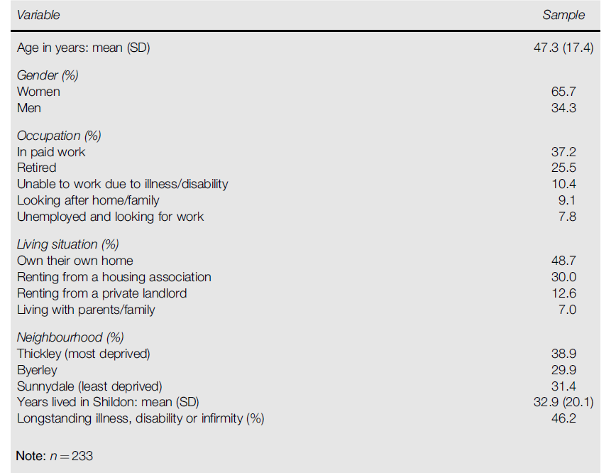
Table 1
Participant Characteristics
From “Examining Associations between Health, Wellbeing and Social Capital: Findings from a Survey Developed and Conducted using Participatory Action Research,” by S. Visram, S. Smith, N. Connor, G. Greig, & C. Scorer, 2018, Journal of Public Mental Health , 17 (3), p. 127 (https://doi.org/10.1108/JPMH-09-2017-0035). Copyright 2018 by Emerald Publishing Limited.
This data was obtained from a sample of people who live in a particular city, and the sample size is \(233\) (as indicated by the \(n = 233\) at the bottom of the table). Moreover, there are two different types of variables summarised in this table:
- categorical variables, for data grouped into categories (the ‘Gender’ variable for example), and
- continuous variables, for numerical data (the ‘Age in years’ variable for example).
These two types of variables need to, and have been, analysed differently. Let’s look at the categorical variables first.
Interpreting descriptive statistics for categorical variables
The categorical variables in this example have been summarised using percentages, and these show what percentage of the sample is in each category for the given variable (note that frequencies are sometimes used instead of percentages, and that these show how many are in each category instead). For example, the descriptive statistics for the ‘Gender’ variable show that \(65.7\%\) of the sample described in Table 1 are women and \(34.3\%\) are men.
If you would like to learn more about descriptive statistics for categorical variables, including how to calculate them, please refer to the Descriptive statistics for one categorical variable section of this module. Otherwise, to practise interpreting descriptive statistics for categorical variables have a go at the following question.
What percentage of the sample described in Table 1 are in each of the categories for the ‘Living situation’ variable?
ANSWER: \(48.7\%\) own their own home; \(30\%\) rent from a housing association; \(12.6\%\) rent from a landlord; \(7\%\) live with parents/family.
Interpreting descriptive statistics for continuous variables
The continuous variables in this example have been summarised using two measures, the first being the mean (also called the arithmetic average). This is the most commonly used measure of central tendency, and is a single value used to describe the data set by indicating the central value. For example, in Table 1 the mean for the ‘Age in years’ variable is \(47.3\), indicating that the average (or central) age of the sample of \(233\) people is \(47.3\). The second measure is the standard deviation (SD), which is the most commonly used measure of dispersion. This is a single value used to describe the data set by indicating how varied (or spread out) it is. The standard deviation for the ‘Age in years’ variable in Table 1 is \(17.4\). This is quite large relative to the mean, indicating that the variability in the ages of the sample of \(233\) people is quite large.
Summarising continuous variables using both a measure of central tendency and a measure of dispersion in this way is optimal, as one without the other does not fully describe the variable. For example, if we were only provided with \(47.3\) as the mean age of the sample then we would have no way of knowing whether everyone in the sample was \(47.3\), or whether the ages of the people in the sample were widely dispersed either side of \(47.3\). Likewise, if we were only provided with the standard deviation of \(17.4\) then we would have no way of knowing the central value of the data set.
It is important to note that the mean and standard deviation are not the only measures of central tendency and dispersion respectively though, and that they are not suitable for use in all situations. In particular when, the data set is skewed (not normally distributed; more on this later) or has outliers (a value or values that are well above or below the majority of the data) the mean and standard deviation do not accurately describe the data. For example, suppose that the vast majority of residents described in Table 1 are aged between \(40\) and \(45\), but that there is a very small group of residents aged in their \(80\)s. The latter ages would be outliers, and would cause the mean to increase above what would otherwise be the central value. In such instances the median is a more appropriate measure of central tendency (as it is not affected by outliers or skew), and the interquartile range is the accompanying measure of dispersion. So if a variable is skewed or has outliers a good piece of research will make use of the median and interquartile range as the summary measures instead.
If you would like to learn more about descriptive statistics for continuous variables, including how to calculate them, please refer to the Descriptive statistics for one continuous variable section of this module. Otherwise, to practise interpreting descriptive statistics for continuous variables have a go at the following question.
Which other continuous variable (aside from ‘Age in years’) has been summarised in Table 1, and what is its mean and standard deviation?
ANSWER: ‘Years lived in Shildon’; mean is \(32.9\) years and standard deviation is \(20.1\) years.
Interpreting inferential statistics
Inferential statistics are used to draw inferences about the wider population when data is obtained from a sample of that population, rather than from the whole population (as the latter is usually not feasible). There are lots of different inferential statistical tests, for different kinds of analysis and for different kinds of variables. For example, different tests are used for continuous and categorical variables and different tests are used for continuous variables depending on their sample size or distribution (pattern or spread of the data).
One example of a distribution that may influence the type of test used is the normal distribution. This is a special kind of distribution that large amounts of naturally occurring continuous data often approximates, and which has two key properties; that the mean, median and mode are all equal, and that fixed proportions of the data lie within certain standard deviations of the mean (\(68\%\) within one SD, \(95\%\) within two SDs and \(99.7\%\) within three SDs). When the sample size is small (typically considered below about 30), or sometimes even when it isn’t, researchers will check to see if continuous variables conform to this distribution. While this isn’t always reported on, when it is the Shapiro-Wilk test (one of a series of tests used for checking normality) is usually referred to.
If an article states that variables pass this test (or more specifically, that the \(p\) value for this hypothesis test is above \(.05\)) it means that normality can be assumed. For example, Power et al. (2019) reference this when they state that the “outcomes were assessed for normality using Shapiro-Wilk” (p. 5). Other times an article might state that variables have been transformed (with a natural logarithm for example), which means that while the variables were not originally normally distributed, they have had a mathematical function applied to them which has made them so (if you would like more information on the properties of the normal distribution, and how to assess whether a variable is normally distributed, please refer to The normal distribution page of this module).
If continuous variables are normally distributed or can be transformed so that they are, or if the sample size is large enough for this not to be an issue, parametric tests are used to analyse them. Alternatively, if the sample size is small and variables are not normally distributed, or if the variables are categorical, nonparametric tests are used instead. Some examples of parametric tests include \(t\) tests, ANOVA and Pearson’s correlation, while some examples of nonparametric tests include chi-square tests, the Mann-Whitney U Test, the Wilcoxon Signed Rank Test, the Kruskal-Wallis One-Way ANOVA and Spearman’s Rho.
For each of these tests, a good article should include statistics that show whether any differences or relationships between variables can be considered statistically and/or practically significant in terms of the population. These terms, the relevant statistics, and how to interpret them are explained below. Alternatively, for more information on inferential statistics, including how to calculate measures of statistical and practical significance, please refer to the Inferential statistics page of this module.
Interpreting statistical significance
Statistical significance refers to the likelihood that what has been observed in the sample (for example a difference in means or a relationship between variables) could have occurred due to random chance alone. In particular, if it is very unlikely that it could have been due to chance alone then it is considered statistically significant in the population. What do we mean by ‘very unlikely’ though? This is where the \(p\) value comes in!
The \(p\) value is the probability that what has been observed could be due to random chance alone, so the lower the \(p\) value, the less likely it is that the results are due to chance. Furthermore, the value that is used as the ‘cut-off’ value to decide whether the probability is low enough or not is called the level of significance, and is denoted by \(\alpha\). Different articles may use different levels of significance, but a very common value is \(.05\). In this case, a \(p\) value less than or equal to \(.05\) means that the results are statistically significant. Other common levels of significance used are \(.01\) and \(.001\), and the article may state what level of significance the results are statistically significant at (for example, that they are statistically significant at the \(.05\) or \(.01\) level).
Note that articles will also often include confidence intervals in addition to \(p\) values. These are ranges of values that a population statistic is expected to lie between with a given level of certainty, which is usually \(95\%\) (in which case it is referred to as a \(95\%\) confidence interval). Confidence intervals can also be used to determine statistical significance (at the \(.05\) level of significance for a \(95\%\) confidence interval), and have the added benefit of providing extra information (for example, the magnitude and direction of a difference between means).
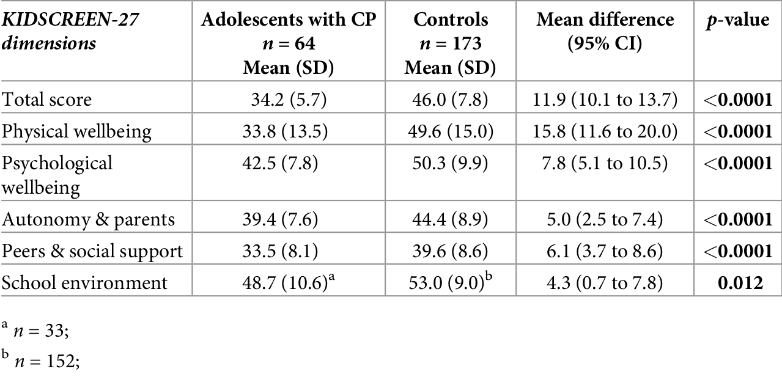
As an example of both \(p\) values and confidence intervals consider Table 2, which displays descriptive statistics together with \(p\) values and confidence intervals for a series of variables. The latter two statistics enable us to determine if there is a statistically significant difference in means between the two groups (adolescents with and without cerebral palsy) at the .05 level of significance for each of the variables.
Table 2
Descriptive statistics, \(95\%\) CIs and \(p\) values for a study investigating mental and physical health of adults with cerebral palsy
From “Health-Related Quality of Life and Mental Health of Adolescents with Cerebral Palsy in Rural Bangladesh,” by R. Power, M. Muhit, E. Heanoy, T. Karim, N. Badawi, R. Akhter, & G. Khandaker, 2019, PLOS One , 14 (6), p. 9 (https://doi.org/10.1371/journal.pone.0217675). CC-BY.
As an example let’s consider at the ‘Total score’ variable, which is the total score on a questionnaire regarding health-related quality of life. The mean difference of \(11.9\) is the difference in ‘Total score’ means between those with cerebral palsy and those without in the sample, and this is a descriptive statistic. The \(95\%\) confidence interval of \(10.1\) to \(13.7\) indicates that we are \(95\%\) confident the sample has come from a population where the difference in means is somewhere between \(10.1\) and \(13.7\), and the fact that this \(95\%\) confidence interval does not include the value of \(0\) (which would indicate no difference in the means) indicates that the difference in means between the two groups is statistically significant at the \(.05\) level of significance.
The fact that \(p < .0001\) also tells us that the difference in means between the two groups is statistically significant, not only at the \(.05\) level of significance but even at the \(.0001\) level of significance. The statistics for the remaining variables can be analysed in the same way; to practise doing this, have a go at the following questions.
Within which range of values is the difference in means for the ‘Peer and social support’ variable expected to lie with \(95\%\) certainty? Does this indicate that the difference in means is statistically significant at the \(.05\) level of significance?
ANSWER: The difference is expected to lie between \(3.7\) and \(8.6\) with \(95\%\) certainty; as this range does not include \(0\) it indicates that the difference is statistically significant at the \(5\%\) level of significance.
Is the difference in means statistically significant for the ‘School environment’ variable at the \(.05\) level of significance? What about at the \(.01\) level of significance?
ANSWER: It is statistically significant at the \(.05\) level of significance, as \(p < .05\) and the confidence interval does not contain \(0\), but not at the \(.01\) level of significance as \(p > .01\).
Interpreting practical significance
Practical significance refers to whether something observed in a sample (for example a difference in means or a relationship between variables) is meaningful in a practical sense or not. It is determined by calculating an effect size , which is different for different tests. For example:
- Cohen’s d is a measure of effect size for \(t\) tests
- Pearson’s correlation coefficient is a measure of effect size for Pearson’s correlation
- Phi, Cramer’s V, odds ratio and relative risk are common measures of effect size for the chi-square test of independence.
Articles that report on practical significance provide an important additional perspective to those that only report on statistical significance, as the latter alone does not allow the reader to have an appreciation of whether the findings are important in a real-life sense or not. In particular, the fact that statistical significance is influenced by sample size means that in very large samples, very small differences that are not actually meaningful in real life may be found to be statistically significant, and conversely in very small samples, very large differences that are meaningful in real life may not be found to be statistically significant. This relates to the statistical power of a test, which is the probability that an effect of a certain size will be found to be statistically significant. In particular, a calculation can be performed to determine how big a sample needs to be in order to observe an effect of a certain size at a certain level of significance for a given power (usually \(0.8\) or above), so articles may also refer to the power of a test.
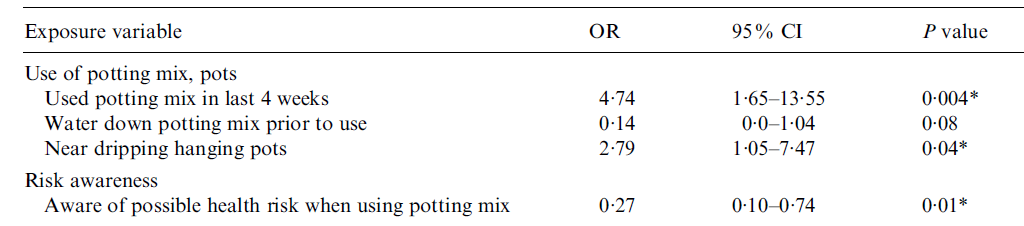
Returning to measures of effect size, and as an example consider Table 3 which shows odds ratios in addition to \(95\%\) confidence intervals and \(p\) values. The latter two relate to the statistical significance of the association between each exposure variable and the outcome variable (L.longbeachae infection), while the odds ratios relate to the practical significance of the association.
Table 3
Odds ratios, \(95\%\) CIs and \(p\) values for a study investigating L.longbeachae infection exposures involving potting mix
From “Does using Potting Mix make you Sick? Results from a Legionella Longbeachae Case-Control Study in South Australia,” by B. A. O’Connor, J. Carman, K. Eckert, G. Tucker, R. Givney, & S. Cameron, 2007, Epidemiology and Infection , 135 (1), p. 36 (https://doi.org/10.1017/S095026880600656X). Copyright 2006 by Cambridge University Press.
For each exposure variable listed, the odds ratio compares the odds of exposure (relative to non-exposure) in the group with L.longbeachae infection, with the odds of exposure (relative to non-exposure) in the group without L.longbeachae infection. In other words, each odds ratio specifies how many times more or less likely those with L.longbeachae infection were to have the exposure than those without L.Longbeachae infection. An odds ratio less than \(1\) means that the group with the L.longbeachae infection are less likely to have the exposure, an odds ratio of \(1\) means that the two groups are equally likely to have the exposure, and an odds ratio greater than \(1\) means that the group with the L.longbeachae infection are more likely to have the exposure.
For example, the first odds ratio of \(4.74\) indicates that those infected with L.longbeachae were \(4.74\) times more likely to have used potting mix in the last four weeks than those not infected. According to Cohen’s conventions for interpreting effect size detailed here, this indicates a medium to large effect (although note that this kind of interpretation is contextual and that interpreting practical significance is less concerned with comparing to cut-off values than statistical significance).
Furthermore, the first \(95\%\) confidence interval of \(1.65 - 13.55\) indicates that we are \(95\%\) confident that this sample comes from a population where those infected with L.longbeachae were somewhere between \(1.65\) and \(13.55\) times more likely to have used potting mix in the last four weeks than those not infected. As this confidence interval does not include the value of \(1\) (which for an odds ratio means that the odds of exposure are the same for those with and without the outcome), the association between using potting mix in the last four weeks and L.longbeachae infection is statistically significant at the \(.05\) level of significance. This is also evidenced by the \(p\) value of \(.004\).
Note that articles will often include adjusted odds ratios in addition to, or in place of, the (crude) odds ratios seen above. These are odds ratios that have been adjusted to take into account any additional confounding variables (i.e. other variables that may be having an influence on the outcome variable), and can be interpreted in the same way.
If you would like to practise interpreting some of the other odds ratios in the table, have a go at the following questions.
How many times more or less likely were those infected with L.longbeachae to be near dripping hanging pots, compared to those not infected? Is this a statistically significant association at the \(.05\) level of significance?
ANSWER: Those infected were \(2.79\) times more likely to be near dripping hanging pots, compared to those not infected with L.longbeachae. This is a statistically significant association at the \(.05\) level of significance as the \(95\%\) confidence interval does not include \(1\) and the \(p\) value is less than \(.05\).
How many times more or less likely were those infected with L.longbeachae to water down potting mix prior to use, compared to those not infected? Is this a statistically significant association at the \(.05\) level of significance?
ANSWER: Those infected were \(0.14\) times as likely to water down potting mix prior to use, compared to those not infected with L.longbeachae. Since the odds ratio is less than \(1\) this is usually expressed as a percentage less likely, which in this case is \(86\%\) (since \(1 - 0.14 = 0.86\)). This is not a statistically significant association at the \(.05\) level of significance as the \(95\%\) confidence interval includes \(1\) and the \(p\) value is greater than \(.05\).
Further example: interpreting one-way ANOVA
As another example of interpreting statistical and practical significance, consider Tables 4 and 5. These show the results of two one-way ANOVAs, used to test for significant differences in mean ‘school attachment scores’ between students of different ages and between students of different socio-economic statuses respectively.
Table 4
Descriptive statistics and one-way ANOVA statistics for a study investigating differences in school attachment scores between age groups
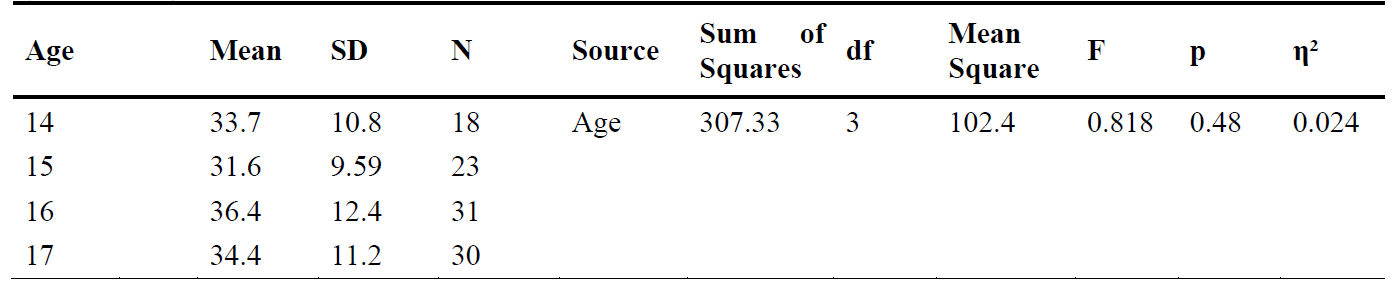
Table 5
Descriptive statistics and one-way ANOVA statistics for a study investigating differences in school attachment scores between socio-economic groups

From “School Attachment and Video Game Addiction of Adolescents with Divorced vs. Married Parents,” by B. TAS, 2019, TOJET: The Turkish Online Journal of Educational Technology , 18 (2), pp. 99-100 (https://files.eric.ed.gov/fulltext/EJ1211160.pdf). Copyright 2019 by The Turkish Online Journal of Educational Technology.
The \(p\) value for each one-way ANOVA indicates either that there is a statistically significant difference between the means of at least two of the groups (if \(p\) is less than or equal to the level of significance), or that there is no statistically significant difference in the means between any of the groups (if \(p\) is greater than the level of significance). Note that if a one-way ANOVA is statistically significant further information is needed, and should be provided, to determine which groups are significantly different from each other. This will either be the results of a planned or post hoc comparison, both of which will provide further \(p\) values which can be interpreted in the usual way.
These tables also include (amongst other statistics) an \(F\) value for each one-way ANOVA. This is the test statistic for this test (note that results of other tests will sometimes include the test value as well; a \(t\) value for a \(t\) test or chi-square value for a chi-square test of independence, for example). This \(F\) value is the ratio of the variability between groups to the variability within each group. For example, an \(F\) value of \(0.818\) for the ‘Age’ variable indicates that the variability in school attachment scores between the four age groups is \(0.818\) times the variability in school attachment scores within each age group (i.e. the variability between the groups is actually less than the variability within the groups). The bigger than \(1\) the \(F\) value is, the greater the likelihood that there is a significant difference in the means between at least two of the groups. However, note that it is the \(p\) value that needs to be interpreted in order to test this.
Lastly, the tables also include eta-squared (\(\eta^2\)) values as measures of effect size, which indicate how much variability (as a percentage) in the school attachment scores can be attributed to age and socio-economic status respectively. For example, the \(\eta^2\) value of \(0.024\) indicates that \(2.4\%\) of the variability in the school attachment scores can be attributed to age. Cohen (1988) suggests that an \(\eta^2\) value of \(.01\) be considered a small effect, \(.059\) be considered a medium effect and \(.138\) be considered a large effect.
Use the information above to answer the following questions:
Is there a statistically significant difference between the mean school attachment scores for any of the four age groups at the \(.05\) level of significance?
ANSWER: No, as the \(p\) value is greater than \(.05\) (\(p = .48\)).
How many times greater is the variability in school attachment scores between the three socio-economic groups, than the variability in school attachment scores within each socio-economic group?
ANSWER: The variability in school attachment scores between the three socio-economic groups is \(2.666\) times the variability in school attachment scores within each socio-economic group.
How much variability (as a percentage) in the school attachment scores can be attributed to socio-economic group?
ANSWER: \(5.1\%\) of the variability in the school attachment scores can be attributed to socio-economic group.
References
Cohen, J. (1988). Statistical power analysis for the behavioral sciences (2nd ed.). Lawrence Erlbaum Associates, Inc.
Connor, B.A., Carman, J., Eckert, K., Tucker, G., Givney, R., & Cameron, S. (2007). Does using potting mix make you sick? Results from a Legionella longbeachae case-control study in South Australia. Epidemiology and Infection, 135 (1), 34-39. https://doi.org/10.1017/S095026880600656X
Power, R., Muhit, M., Heanoy, E., Karim, T., Badawi, N., Akhter, R., & Khandaker, G. (2019). Health-related quality of life and mental health of adolescents with cerebral palsy in rural Bangladesh. PLoS One, 14 (6), 1-17. https://doi.org/10.1371/journal.pone.0217675
TAS, B. (2019). School attachment and video game addiction of adolescents with divorced vs. married parents. TOJET : The Turkish Online Journal of Educational Technology , 18 (2), 93-106. https://files.eric.ed.gov/fulltext/EJ1211160.pdf
Visram, S., Smith, S., Connor, N., Greig, G., & Scorer, C. (2018). Examining associations between health, wellbeing and social capital: Findings from a survey developed and conducted using participatory action research. Journal of Public Mental Health, 17 (3), 122-134. https://doi.org/10.1108/JPMH-09-2017-0035 Descriptive statistics
Descriptive statistics are used to summarise and describe a variable or variables for a sample of data (as opposed to drawing conclusions about any larger population from which the sample was drawn, which is covered in the Inferential statistics page). For example, sample statistics such as the mean (\(\bar{x}\)) and standard deviation (\(s\)) are often used to summarise and describe continuous variables.
Furthermore, descriptive statistics can be used to summarise just one variable at a time (univariate analysis), to analyse relationships between two variables (bivariate analysis) and, in some cases, to describe patterns across three or more variables (multivariate analysis, which is not covered here).
This page details ways of displaying and of using descriptive statistics to perform univariate and bivariate analysis, for both categorical and continuous data.
In brief, it covers the following:
- How to display data for one categorical variable
- How to use descriptive statistics to analyse data for one categorical variable
- How to display data for one continuous variable
- How to use descriptive statistics to analyse data for one continuous variable
- How to compare means of a continuous variable between different groups
- How to display data for two categorical variables
- How to use descriptive statistics to analyse data for two categorical variables
- How to display data for two continuous variables
- How to use descriptive statistics to analyse data for two continuous variables
</div>
Displaying data for one categorical variable
One way of displaying data for a single categorical variable is by using a table, or in particular a frequency distribution table. This is a table which displays the various categories for a variable, along with the corresponding frequencies (i.e. how often each category occurs in the data) and usually associated percentages (sometimes including cumulative percentages, which give the sum of all the percentages up to and including that row of the table).
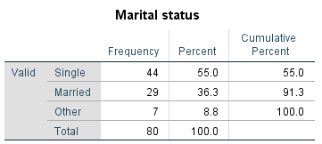
For example, the following is a frequency distribution table showing the frequency of each category of marital status in a sample of 80 people, along with the corresponding percentages:
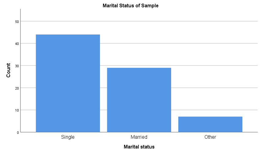
Another way to display categorical data for a single variable is using a column graph or bar chart. Column graphs and bar charts use rectangles of equal width (which do not touch) to represent each data category. The rectangles are drawn vertically for column graphs and horizontally for bar charts, and in each case the height (or length) of the rectangles allows the various quantities for each category to be compared, typically as counts or percentages. For example:
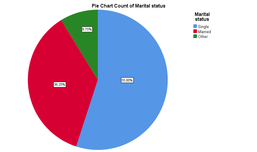
Categorical data for a single variable is also sometimes displayed in a pie chart, in order to show how the sample is divided up between the various categories. For example the data for marital status could be displayed in a pie chart as follows:
Descriptive statistics for one categorical variable
Descriptive statistics used to analyse data for a single categorical variable include frequencies, percentages, fractions and/or relative frequencies (which are simply frequencies divided by the sample size) obtained from the variable’s frequency distribution table.
For example, we can describe the sample of data for the marital status variable from the previous section by selecting some key values from its frequency distribution table, such as:
- \(91.3\%\) of the sample are either single or married
- \(7\) people in the sample identified their marital status as ‘other’
- the relative frequency of people in the sample who are married is \(0.36\)
- over \(\frac{1}{2}\) of the people in the sample are single.
If you would like to practise analysing data for a single categorical variable, have a go at the following activity.
Displaying data for one continuous variable
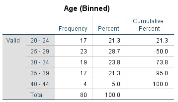
Continuous data for a single variable can also be displayed in a frequency distribution table, but the data first needs to be grouped into bins (also known as class intervals). These should be chosen based on the data, but they should generally be of the same size and ideally there should not be too many.
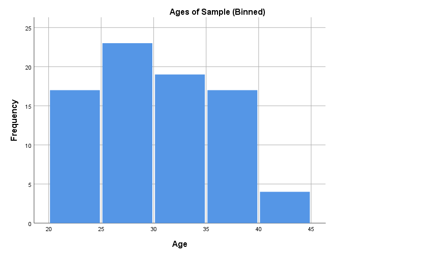
For example, the following is a frequency distribution table showing the frequency of ages of a sample of 80 people, once they have been sorted into bins:
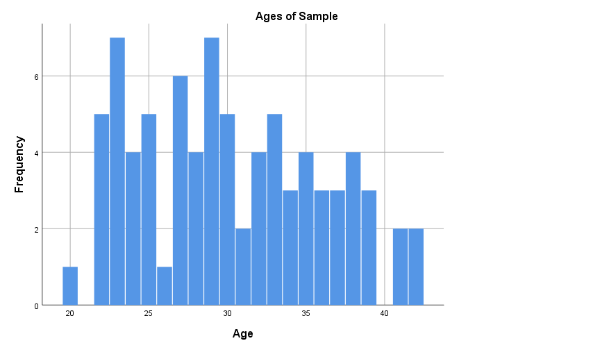
As for graphs that display continuous data for a single variable, one of the most commonly used is a histogram. These have the following properties:
- as the variable is continuous the bars touch (unless an interval has zero frequency)
- the bars are vertical
- the vertical axis should start at zero and should have no breaks
- the area of each bar represents the frequency of the corresponding bin.
Note that different versions of a histogram can be created for the same variable, depending on the bin (class interval) width used. For example, the first histogram below uses bins of width one, while the second uses the bins as shown in the frequency distribution table above. The software you use to produce your histogram will typically decide this for you, so it is not something to be overly concerned about, but if you are wanting to create or manipulate your own histogram keep in mind it is just a matter of choosing a bin width in accordance with the level of detail you wish to show:
Another graph used to display continuous data for a single variable is a box plot (also called a box and whisker plot), which is a diagram showing the way the data for a variable is distributed. For example, a box plot for our Age variable is as follows (click on the plus signs to learn about the key features of the graph, some of which are explained in more detail in the Descriptive statistics for one continuous variable section that follows):
Descriptive statistics for one continuous variable
Continuous data for a single variable is generally analysed using two types of descriptive statistics:
- measures of central tendency, which summarise the data set by finding the average, central or typical member (for example mean, median and mode), and
- measures of dispersion, which summarise the data set by finding out how widely it is spread or dispersed (for example range, interquartile range, variance and standard deviation).
It is important not only to understand how to calculate and interpret the various measures of central tendency and dispersion, but to know when it is appropriate to use the various types. How to do both is explained in the following two sections.
Measures of central tendency
The most common measure of central tendency is the mean (otherwise known as the arithmetic average), which is calculated by adding together all of the data and then dividing through by the total number of values. The sample mean is denoted by \(\bar{x}\), and for a sample of size \(n\) the formula for calculating the mean is written as follows (note that \(\sum\) represents the sum of all the values):
\[\bar{x} = \frac{\sum x}{n}\]For example, the mean of the following sample of ten ages:
\[19, 25, 28, 28, 23, 15, 28, 22, 24, 21\]can be calculated as:
\[\begin{aligned} \bar{x} &= \frac{19+25+28+28+23+15+28+22+24+21}{10} \\\ &= 23.3 \end{aligned}\]While the mean is typically used as the measure of central tendency for continuous data, it may not be appropriate if the data set is badly skewed, contains outliers or if the variable is censored (not fully observed). In these situations the median is more suitable. This is the midpoint of the distribution, which is calculated for a sample by sorting the data from smallest to largest and then finding the middle value (or the mean of the middle two values if there are an even number of observations). For example, putting our sample of ten ages in order gives:
\[15, 19, 21, 22, 23, 24, 25, 28, 28, 28\]and the median is then the mean of the middle two:
\[\frac{(23+24)}{2} = 23.5\]Finally, the mode is the most frequently occurring value (or values) in the sample (if there are two or more values that are equally common we quote them all, rather than finding the average). Note that the mode may not necessarily be anywhere near the middle of the data set, and hence is not necessarily ‘central’, but it is useful when the most common value is of interest. For example, the mode of our sample of ten ages:
\[19, 25, 28, 28, 23, 15, 28, 22, 24, 21\]is \(28\).
Note also that the mode can be, and is most often, used for categorical data.
If you would like to test your understanding of the mean, median and mode, have a go at one or both of the following activities.
Measures of dispersion
The simplest measure of dispersion is the range, which is simply the difference between the smallest and the largest value in the sample. For example, the range of our sample of ten ages in the previous section is \(13\) (i.e. \(28 - 15\)). While the range is easy to calculate, it is usually of limited use as it takes into account just two values in the data set.
A measure of dispersion that takes into account more, if still not all, values in a data set is the calculation of percentiles. These measure position from the beginning of an ordered data set, and can be used to measure the relative standing of a particular observation. For example, stating that a child is in the \(97\)th percentile of a sample for height means that he or she is taller than \(97\%\) of others in the sample. As another example, our sample of ages contains only ten pieces of data so lends itself nicely to calculating percentiles that are multiples of \(10\). Have a look at some of these in the diagram below (click on the plus signs to find out about the different percentiles):
A specific type of percentiles which divide the sample into quarters are quartiles (as shown on the box plot in the previous section). For example, the:
- \(25\)th percentile is known as the first or lower quartile
- \(50\)th percentile is known as the median
- \(75\)th percentile is known as the third or upper quartile.
The quartiles for our sample of age data are as follows (note the different colours for each quarter of the sample, and click on the plus signs to find out about the different quartiles):
Once you have determined the quartiles you can determine another measure of dispersion, called the interquartile range. This is the difference between the first and the third quartiles, which is \(7\) for the example above. The interquartile range is quoted in conjunction with the median in situations where the latter is more appropriate than the mean.
In all other situations the mean and standard deviation are usually used to summarise a sample. The standard deviation takes into account all of the values in a sample, and is calculated by finding the deviation of each value from the mean, squaring the result, then adding them all together and dividing by one less than the sample size. This gives yet another measure of dispersion, known as the variance, and then taking the positive square root of this gives the standard deviation. The standard deviation is generally more relevant than the variance, as it is measured on the original scale of the data. The formula for the standard deviation (\(s\)) of a sample of size \(n\) is:
\[s =\sqrt{\frac{\sum(x - \bar{x})^2}{n - 1}}\]While standard deviation (along with other measures of dispersion and central tendency) can be calculated using various software, it is also good to understand how to determine it manually. For example, to calculate the standard deviation of our ten ages:
\[19, 25, 28, 28, 23, 15, 28, 22, 24, 21\]we first need to find the mean of the sample (\(\bar{x}\)), which we know to be \(23.3\).
Next, calculating the deviation of each age from this mean gives:
\[-4.3, 1.7, 4.7, 4.7, -0.3, -8.3, 4.7, -1.3, 0.7, -2.3\]and squaring these gives:
\[18.49, 2.89, 22.09, 22.09, 0.09, 68.89, 22.09, 1.69, 0.49, 5.29\]Now adding these ten values gives a total of \(164.1\), and diving through by \(9 \) (i.e. \(10 - 1\)) gives \(18.23\). Finally, taking the square root gives the sample standard deviation of \(4.27\)
If you would like to practise calculating the range, interquartile range, variance and standard deviation, and to practise deciding which measure of central tendency and measure of dispersion to interpret, have a go at the following activities.
Comparing means
Measures of central tendency and dispersion can also be used to test for differences in a continuous variable between different categories of a categorical variable. This is often done to compare means between groups.
For example, if we know that the first five people in our sample of ages are females and the second five people are males, we can compare the means of the two groups:
\[\begin{aligned} \textrm{Ages of females} &= 19, 25, 28, 28, 23 & \textrm{Mean age of females} = & 24.6 \\\ \textrm{Ages of males} &= 15, 28, 22, 24, 21 & \textrm{Mean age of males} = & 22 \end{aligned}\]So the mean of the females in our sample is \(2.6\) years greater than the mean of the males.
If you would like to practise comparing means, have a go at the following activity.
Displaying data for two categorical variables
Cross-tabulations (or contingency tables) are used to investigate associations between two categorical variables for a sample. A cross-tabulation contains multiple rows and columns, with the categories of the independent variable in the rows and the categories of the dependent variable in the columns. Each cell of the table contains the frequency or number of subjects that fall into the combination of categories of the two variables, subtotals are given for each column and row, and a final total is given in the bottom right-hand corner of the table.
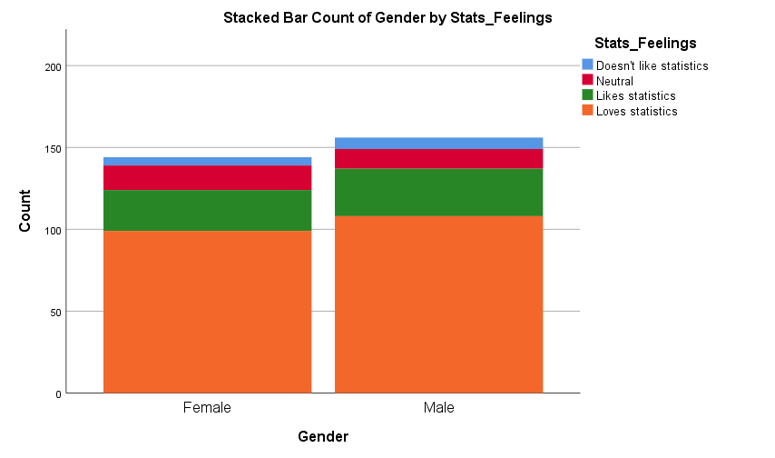
For example, the following cross-tabulation displays data for two variables (gender and feelings towards statistics), for a (fictional) sample of 300 people:
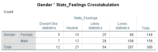
Cross-tabulations also often include row, column and/or total percentages as applicable. To find out about these, click on the plus signs in the diagram below:
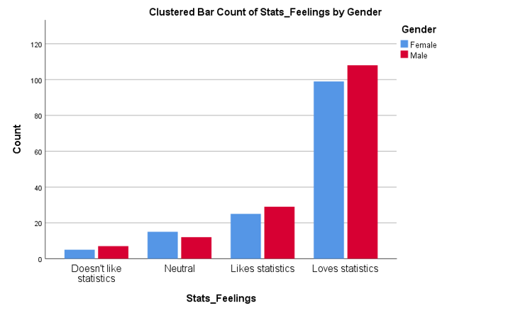
Data for two categorical variables can also be displayed in either a clustered or stacked bar chart. A clustered bar chart is great for comparing each category of one variable between the different categories of the other variable, while a stacked bar chart is better for comparing the total for each of the categories for one of the variables.
Descriptive statistics for two categorical variables
Data in cross-tabulations can be analysed using the frequencies and percentages shown previously. In addition, expected frequencies can also be used to analyse the association between the variables in the sample. These frequencies are calculated based on the assumption that there is no association between the variables in the sample, and can be compared to actual frequencies to test for association. In particular, the closer the expected and the actual frequencies are to each other, the less likely it is that there is an association between them (and therefore the less likely it is that one can be used to predict the other).
For some examples of how expected frequencies are calculated, and how they can be interpreted, click on the plus signs in the diagram below:
If you would like to practise interpreting cross-tabulations, have a go at one or both of the following activities.
Displaying data for two continuous variables
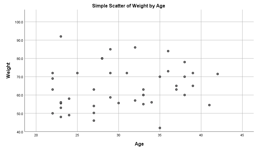
The relationship (or lack of) between two continuous variables in a sample can be visualised in a scatterplot , which plots the independent variable on the x-axis against the dependent variable on the y-axis.
For example, a scatterplot for the ages and weights of a sample of 80 people is shown below. The fact that the data points do not approximate a straight line indicates a weak to non-existent linear relationship between the variables (note that two variables may have a non-linear relationship between them, but non-linear relationships are not covered in this module).
In terms of linear relationships, you can use a scatterplot to observe:
- the strength of any linear relationship between the variables, by observing how closely the data points approximate a straight line, and
- the direction of any linear relationship, by observing whether the line approximated by the points slopes up (positive relationship) or down (negative relationship).
Descriptive statistics for two continuous variables
Finally, note that the strength and direction of a linear relationship (or lack of) between two continuous variables can be quantified by Pearson’s correlation coefficient (\(r\)).
The correlation coefficient is a number between \(-1\) and \(1\), with negative values indicating a negative linear relationship and positive values indicating a positive linear relationship. Furthermore:
- \(r = 0\) indicates no linear relationship between the variables,
- \(r\) values between \(0\) and \(0.3\) (\(0\) and \(-0.3\)) indicate a weak positive (negative) linear relationship between the variables,
- \(r\) values between \(0.3\) and \(0.7\) (\(-0.3\) and \(-0.7\)) indicate a moderate positive (negative) linear relationship between the variables,
- \(r\) values between \(0.7\) and \(1\) (\(-0.7\) and -\(1\)) indicate a strong positive (negative) linear relationship between the variables, and
- \(r = 1\) (\(-1\)) indicates a perfect positive (negative) linear relationship between the variables.
For example if two variables that contain data for age and scores on a memory test have a correlation coefficient (\(r\) value) of \(-.72\), it indicates that there is a strong, negative linear relationship between them.
For practise interpreting a correlation coefficient together with a scatterplot, have a go at the following activity.
H5P interactive activity
The normal distribution
Many of the statistical tests detailed in subsequent pages of this module rely on the assumption that any continuous data approximates a normal distribution, or that the sample size is large enough that the sampling distribution of the mean approximates a normal distribution. But what exactly are the normal and sampling distributions, how large is a large enough sample and how do you know if a continuous variable is normally distributed? This page will address these questions, and is an important precursor to the content on inferential statistics covered in the following pages.
In brief, it covers the following:
- The definition of the normal distribution
- The definition of the sampling distribution
- How to test for normality
- Options for transforming variables if they are not normally distributed
</div>
The normal distribution
The normal distribution is a special kind of distribution that large amounts of naturally occurring continuous data (and hence also smaller samples of such data) often approximates. As a result, properties of the normal distribution are the underlying basis of calculations for many inferential statistical tests, called parametric tests. These key properties are as follows:
- The mean, median and mode are all equal in a normal distribution.
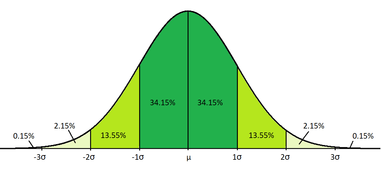
- Fixed proportions of the data lie within certain numbers of standard deviations from the mean in a normal distribution. In particular, 68% of the data lies within one standard deviation, 95% lies within two standard deviations and 99.7% lies within three standard deviations.
Given these properties, the graph of a normally distributed variable has a bell shape as shown below. Note that the percentages displayed here are given to two decimal places, while the percentages above are rounded values. Also note that the \(\mu\) and \(\sigma\) symbols represent population mean and population standard deviation respectively:
If you would like to practise interpreting a normally distributed data set, have a go at the following activity.
The sampling distribution
The descriptive statistics covered in the previous page of this module are used to analyse the data you have access to, which in most cases is a random sample of a larger population. It is important to note that a particular random sample from a population is only one of a number of possible samples though, and that values for sample statistics (e.g. the sample mean) can, in theory, be calculated for each possible sample of the same size. For example, we could measure the heights of a random sample of 100 Curtin students and obtain a mean of that sample, then we could do the same for a different random sample of 100 Curtin students, and for another sample, and so on and so on to calculate means for each possible sample of the same size.
All of these sample statistics (e.g. all of the means for our height example) have a distribution of their own, which is known as the sampling distribution. We could visualise this distribution using a histogram (as per any other data) if we had access to all the data, but note you wouldn’t usually do this as it would defeat the purpose of obtaining a random sample! Instead, inferential statistics estimate properties of the sampling distribution using data obtained from one random sample. The sampling distribution is therefore an important concept to be familiar with, and in particular it is important to be aware of these key properties of the sampling distribution of the mean:
- As the sample size increases, the shape of the sampling distribution of the mean becomes increasingly similar to the normal distribution. This is a very important theorem in statistics, and is called the Central Limit Theorem. Generally a sample size of 30 or more is considered large enough for the sampling distribution to approximate a normal distribution (although if the variable’s distribution is very skewed, a larger sample size may be required), and for this reason a sample size of 30 or more is usually enough to fulfil any normality requirements.
- The mean of the sampling distribution equals the mean of the population.
- The standard deviation of the sampling distribution equals the standard deviation of the population divided by the square root of the sample size. This is the standard error of the mean.
Testing for normality
If the inferential statistical test you wish to conduct requires a normally distributed continuous variable (or variables) and your sample size is not sufficiently large (typically 30 or above), then you will need to test to determine whether or not this is the case. Unfortunately there is not a single yes-or-no test for normality, and rather it requires assessing up to eight different factors in order to determine if the data approximates the normal distribution ‘closely enough’ (the data will never be perfectly normally distributed, and often a fair bit of deviation is acceptable). While some of these tests are more commonly used than others it is a good idea to evaluate as many as possible, particularly when you are first getting started, as the more information you have means the more complete of a picture you will have of your data, and the more well-informed your conclusion will be.
The eight statistics and graphs you can interpret are as follows:
-
Mean, median and mode
For a perfect normal distribution these three values should all be the same, so checking whether they are similar is a good (and simple) way to start. Note however that even in normally distributed data the mode may sometimes be higher or lower, but this is less of a concern than any differences between the mean and median. -
Skewness
Skewness measures the symmetry of the distribution. A skewness of \(0\) indicates a perfectly symmetrical distribution, while a negative value indicates negative skew (long tail to the left) and a positive value indicates positive skew (long tail to the right). If the data approximates a normal distribution the skewness should be close to \(0\), but a value within the range of \(-1\) to \(1\) is considered acceptable. Additionally, the z-score for the skewness, which can be calculated by dividing the skewness by its standard error, should be within the range of \(-1.96\) to \(1.96\) -
Kurtosis
Kurtosis measures the heaviness of the distribution’s tails. The kurtosis for the normal distribution is \(3\), although many researchers and software programs (e.g. SPSS) actually provide the excess kurtosis instead. This is calculated by subtracting \(3\) from the kurtosis, giving the normal distribution a value of \(0\). Using this measure, a positive kurtosis indicates wider tails and a negative kurtosis indicates narrower tails, but again a value within the range of \(−1\) to \(1\) is considered acceptable. Additionally, the z-score for the (excess) kurtosis, which can be calculated by dividing the (excess) kurtosis by its standard error, should be within the range of \(-1.96\) to \(1.96\) -
Normality test (e.g. Shapiro-Wilk)
The Shapiro-Wilk test is a normality test, which tests the null hypothesis that the distribution approximates a normal distribution (another normality test is the Kolmogorov-Smirnov test). A significance (\(p\)) value greater than \(0.05\) indicates that this null hypothesis should not be rejected, and therefore provides evidence that a normal distribution can be assumed (more on hypothesis testing is covered in the Inferential statistics page of this module). Note that this test is generally only used for sample sizes less than \(100\), as it can be too sensitive for larger samples. -
Histogram
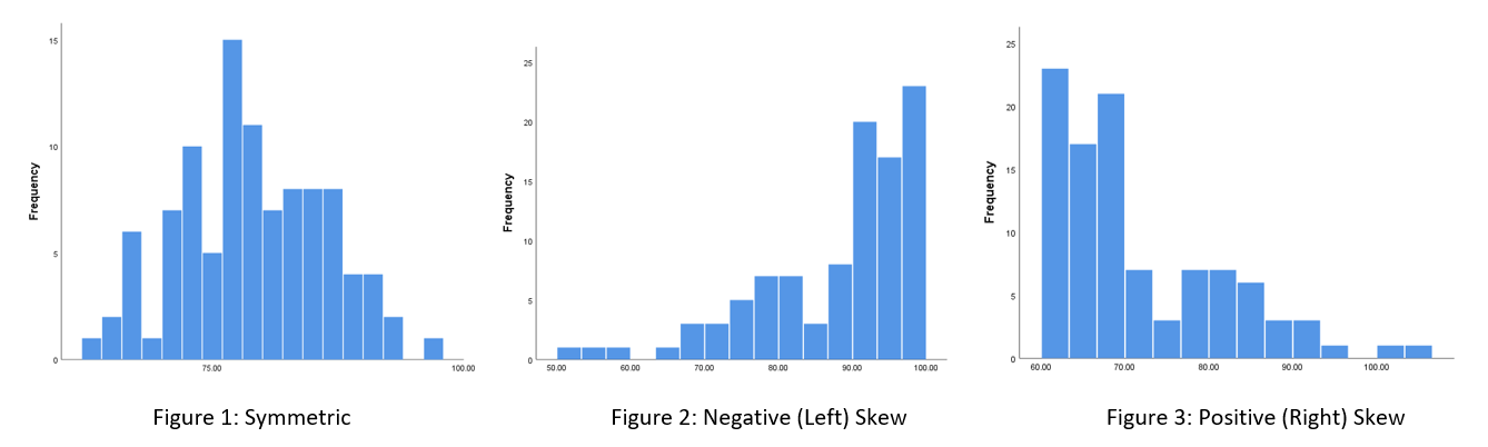
If the data is normally distributed the histogram should be approximately symmetric and centred around the mean (Figure 1). Alternatively, if there is a long tail to the left only it is skewed to the left (negatively skewed) (Figure 2), or if there is a long tail to the right only it is skewed to the right (positively skewed) (Figure 3):
-
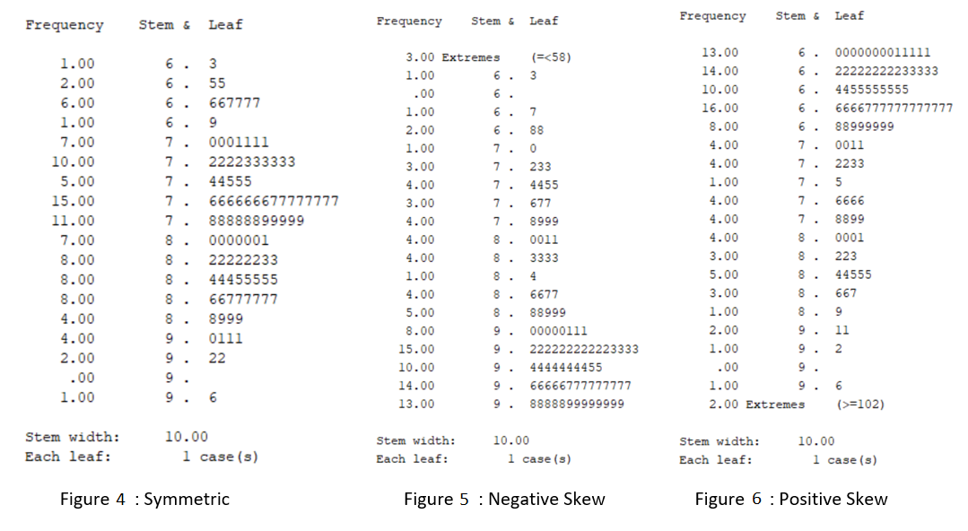
Stem and leaf plot
A stem and leaf plot displays the frequency of each value in the data set, organised into ‘stems’ and ‘leaves’. For example, Figure 4 below shows that there is one value of \(63\), two values of \(65\), six values of either \(66\) or \(67\), etc. This plot can be interpreted in the same way as a histogram, only rotated on its side.
-
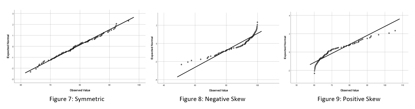
Normal Q-Q plot
If the data is normally distributed the points on a normal Q-Q plot will fall approximately on the straight diagonal line (Figure 7). Otherwise, the points will not lie on the straight diagonal line (Figures 8 and 9). Note that another version of this plot, the detrended Q-Q plot, is sometimes also analysed. In the detrended plot there should be roughly equal number of points above and below the line, with no obvious trend.
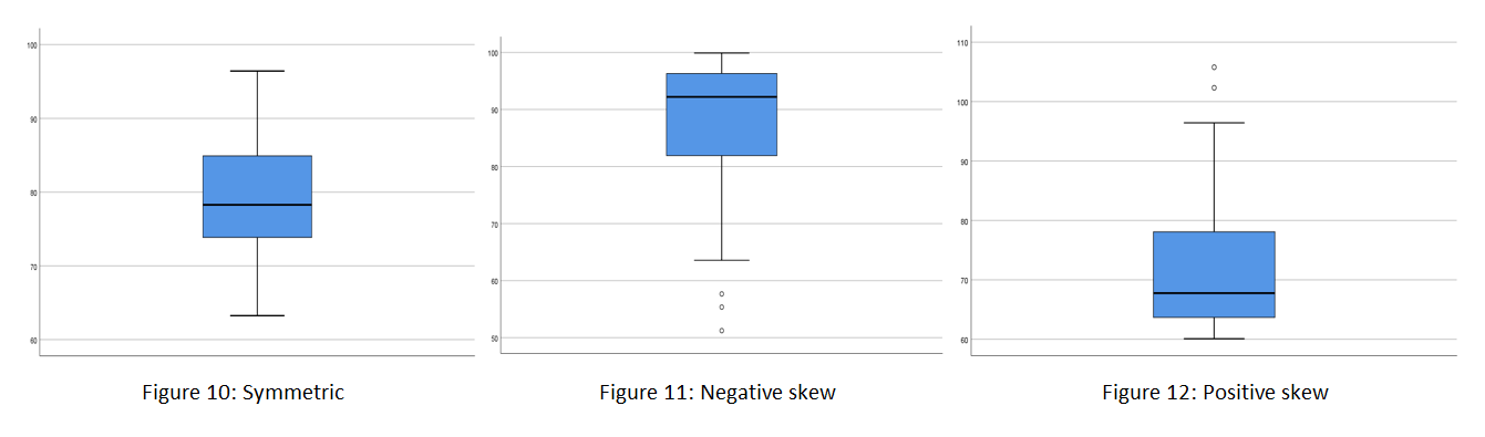
- Boxplot
If the data is normally distributed the median should be positioned approximately in the centre of the box, both whiskers should have similar length and ideally there should be no outliers (Figure 10). Alternatively, the boxplot may display a negative skew (Figure 11) or a positive skew (Figure 12):
After analysing the data relating to these tests of normality, you should come to an overall conclusion based on what the majority of the tests indicate. For example, your conclusion might be that the data is approximately normally distributed, or it might be that it is positively or negatively skewed.
For a worked example of assessing normality, you make like to view the Introduction to SPSS module. You can also practise assessing whether or not data approximates a normal distribution by having a go at the following activity.
Transforming variables
If tests for normality indicate that the variable is not normally distributed (and your sample size is not sufficiently large), you can try transforming the variable to see if it conforms more to the normal distribution. For example, if the data is negatively skewed you could try taking the square of the data, or if it is positively skewed you could try taking the natural logarithm (\(ln\)), the square root or the reciprocal.
Once the data has been transformed, it should be tested again for normality. If the transformation has ‘worked’, any further inferential analysis should be conducted on the transformed data. If it hasn’t, you will need to use non-parametric tests instead. Inferential statistics
So far we have been using descriptive statistics to describe a sample of data, by calculating sample statistics such as \(\bar{x}\) (the sample mean) and \(s\) (the sample standard deviation).
However, research is often conducted with the aim of using these sample statistics to estimate (and compare) true values for populations. The latter are known as population parameters, and are denoted by Greek letters such as \(\mu\) (population mean) and \(\sigma\) (population standard deviation). Inferential statistics allow us to make statements about unknown population parameters based on sample statistics obtained for a random sample of the population. There are two key types of inferential statistics, estimation and hypothesis testing, and these will both be covered in this page.
In brief, it covers the following:
- Using point estimates and confidence intervals for estimation
- How to write hypotheses in order to test for statistical significance
- How to interpret \(p\) values in order to assess statistical significance
- How to interpret practical significance
- The difference between parametric and non-parametric tests
</div>
First, though, you may like to test your understanding of inferential statistics by choosing the best answer to the following question:
Estimation
When sample statistics are used to estimate population parameters, either using a single value (known as a point estimate) or a range of values (known as a confidence interval), it is referred to as estimation. These two different kinds of estimation are covered in more detail in the following sections.
Point estimates
Suppose a researcher is interested in cholesterol levels in a population. If they recruit a sample randomly from the population, they can estimate the cholesterol level of the whole population using the actual cholesterol level they calculated directly from the sample. In this case:
- \(\bar{x}\) (the sample mean cholesterol level) is a point estimate of \(\mu\) (the population mean cholesterol level)
- \(s\) (the sample standard deviation for cholesterol level) is a point estimate of \(\sigma\) (the population standard deviation).
While point estimates are useful, most often it is preferable to estimate a population parameter using a range of values so that the likely variation between the sample and population statistics is taken into account. This is where confidence intervals come in.
Confidence intervals
A confidence interval gives a range of values as an estimate for a population parameter, along with an accompanying confidence coefficient. This is the level of certainty that the interval includes the population parameter, and is typically \(95\%\). For example, a \(95\%\) confidence interval for population mean blood glucose level of (\(4\) mmol/L, \(6\) mmol/L) indicates that we are \(95\%\) certain that the population mean blood glucose level lies between \(4\) mmol/L and \(6\) mmol/L.
For another way of interpreting confidence intervals, think back to the sampling distribution of a sample statistic and consider that you could calculate a confidence interval for each possible sample of the same size. A \(95\%\) (for example) confidence interval means that you would expect 95 out of every 100 of these intervals to contain the population mean.
While confidence intervals can be calculated for a range of statistics, a common example is a confidence interval for the population mean. This can be calculated based on the sampling distribution of the sample mean according to the following formula:
\[\textrm{confidence interval for population mean} = \textrm{sample mean} \pm \textrm{a multiple of the standard error of the mean}\]There are two things to note when using this formula, the first being that the multiple to use depends on the confidence coefficient. For example, a \(95\%\) confidence interval requires a multiple of \(1.96\) (this relates back to the normal distribution, and the fact that \(95\%\) of the area under a normal curve lies within 1.96 standard deviations of the mean). The second thing to note is that the standard error of the mean for a sample of size \(n\) with standard deviation \(s\) is equal to \(\frac{s}{\sqrt{n}}\)
Therefore, the formula to calculate the \(95\%\) confidence interval for the population mean using a sample of size \(n\) with mean \(\bar{x}\) and standard deviation \(s\) becomes:
\[95\% \textrm{ confidence interval for population mean} = \bar{x} \pm 1.96 \times \frac{s}{\sqrt{n}}\]Note that before calculating a confidence interval for a population mean, however, you should ensure the following assumptions are valid:
Assumption 1: The sample is a random sample that is representative of the population.
Assumption 2: The observations are independent, meaning that measurements for one subject have no bearing on any other subject’s measurements.
Assumption 3: The variable is normally distributed, or the sample size is large enough that the sampling distribution of the mean approximates a normal distribution.
</div>
Some important points to note about confidence intervals are as follows:
- The confidence interval for the population mean is symmetric about the sample mean.
- The length of a confidence interval increases for higher levels of confidence.
- The length of a confidence interval is shorter for larger samples than for smaller samples.
- Wider confidence intervals are obtained from variables with larger standard deviations, since more variation in the variable implies less accuracy in estimation.
Finally, it is important to remember that a population parameter is fixed and that it is the sample statistic and confidence interval that change from sample to sample. Once the interval is calculated then the unknown population value is either inside or outside of the interval, and we can only state the certainty with which we believe the interval to contain the population value.
If you would like to practise calculating and interpreting confidence intervals, have a go at one or both of the following activities.
Hypothesis testing
Hypothesis testing involves formulating hypotheses about the population in general based on information observed in a sample. These hypotheses can then be tested to find out whether differences or relationships observed in the sample are statistically significant in terms of the population, or whether they have just occurred due to random chance in the sample.
In order to do this two complementary, contradictory hypotheses need to be formulated, called the null hypothesis and the alternative hypothesis (or research hypothesis). These hypotheses will be formulated differently depending on whether you are conducting a two-tailed hypothesis test (which tests for an effect in either direction) or a one-tailed hypothesis test (which only tests for an effect in one direction). Choosing which test to perform will depend on your methodology, however typically two-tailed tests are used unless there is a reason not to (e.g. if the effect is only possible in one direction). For this reason, we will focus on two-tailed hypothesis tests in this module. These have the following hypotheses:
Null hypothesis (\(\textrm{H}_\textrm{0}\)): This hypothesis states that there is no difference or relationship between variables in a population. For example, no significant difference between two population means, no significant association between two categorical variables, no significant correlation between two continuous variables or no significant difference from the normal distribution (as for Shapiro-Wilk’s test).
</div>
Alternative hypothesis (\(\textrm{H}_\textrm{A}\)): Also known as the research hypothesis, this hypothesis states the opposite of the null hypothesis (i.e. it states that there is a difference or relationship between variables in a population). For example, that there is a significant difference between two population means, a significant association between two categorical variables, a significant correlation between two continuous variables or a significant difference from the normal distribution (as for Shapiro-Wilk’s test).
</div>
Both hypotheses can be written using either words or symbols, often in a few different ways. For example, if we want to test whether there is a significant change in the mean blood pressure of a population of patients after they have take a new medication, some of the different ways we could write null and alternative hypotheses are:
\(\textrm{H}_\textrm{0}\): there is no significant difference in blood pressure before and after the medication
\(\textrm{H}_\textrm{0}: \mu_{\textrm{bp before}} = \mu_{\textrm{bp after}}\)
\(\textrm{H}_\textrm{0}: \mu_{\textrm{bp before}} - \mu_{\textrm{bp after}} = 0\)
\(\textrm{H}_\textrm{A}\): there is a significant difference in blood pressure before and after the medication
\(\textrm{H}_\textrm{A}: \mu_{\textrm{bp before}} \neq \mu_{\textrm{bp after}}\)
\(\textrm{H}_\textrm{A}: \mu_{\textrm{bp before}} - \mu_{\textrm{bp after}} \neq 0\)
If you would like to practise writing hypotheses, have a go at formulating null and alternative hypotheses for the following activity.
You wish to test whether there is a significant difference between the mean before and after heart rates for the population of people who complete a fun run.
\(\textrm{H}_\textrm{0}\): There is no significant difference in heart rate before and after the fun run (\(\mu_{\textrm{hr before}} = \mu_{\textrm{hr after}}\), or \(\mu_{\textrm{hr before}} - \mu_{\textrm{hr after}} = 0\))
\(\textrm{H}_\textrm{A}\): There is a significant difference in heart rate before and after the fun run (\(\mu_{\textrm{hr before}} \neq \mu_{\textrm{hr after}}\), or \(\mu_{\textrm{hr before}} - \mu_{\textrm{hr after}} \neq 0\))
You wish to test whether there is a significant difference in mean overall grades between the populations of male and female students enrolled in a particular unit.
\(\textrm{H}_\textrm{0}\): There is no significant difference in mean grades for male and female students (\(\mu_{\textrm{male}} = \mu_{\textrm{female}}\), or \(\mu_{\textrm{male}} - \mu_{\textrm{female}} = 0\))
\(\textrm{H}_\textrm{A}\): There is a significant difference in mean grades for male and female students (\(\mu_{\textrm{male}} \neq \mu_{\textrm{female}}\), or \(\mu_{\textrm{male}} - \mu_{\textrm{female}} \neq 0\))
You wish to test whether there is a significant correlation between hours of study and exam marks in a population of university students.
\(\textrm{H}_\textrm{0}\): There is no significant correlation between hours of study and exam marks (\(r = 0\))
\(\textrm{H}_\textrm{A}\): There is a significant correlation between hours of study and exam marks (\(r \neq 0\))
Once the hypotheses have been formulated they can be tested to evaluate statistical significance, as explained in the following section. In addition, note that it is important to keep practical significance in mind at this point as well, and that this is explained in the subsequent section.
Statistical significance
An appropriate test needs to be conducted in order to evaluate statistical significance, with some common examples being one sample, paired samples and independent samples \(t\) tests, one-way ANOVA, the chi-square test of independence and Pearson’s correlation (all of which are covered in later pages of this module). Typically you will conduct such a test using statistical software or a programming language (e.g. SPSS, Stata, SAS, R or Python), although you can do it manually if wished (not covered here).
Either way, a test statistic will be calculated which compares the value of the sample statistic (for example, the sample mean change in blood pressure in our blood pressure example) with the value specified by the null hypothesis for the population statistic (for example, a mean change in blood pressure of zero). The name of this test statistic, and how it is calculated, will vary depending on the test you are doing (for example a \(t\) test will calculate a \(t\) value, a one-way ANOVA will calculate an \(F\) value and a chi-square test of independence will calculate a chi-square value), but in each case a large test statistic indicates that there is a large discrepancy between the hypothesised value and the sample statistic.
Furthermore, a \(p\) value (or probability value) will also be calculated for the test (or two \(p\) values may be calculated, a one-sided \(p\) value and a two-sided \(p\) value; in this case the two-sided \(p\) value should be used unless you have previously determined that you will conduct a one-sided hypothesis test). This gives the probability of obtaining the test statistic in question if the null hypothesis is true, and it is this value that is interpreted when deciding whether or not to reject the null hypothesis (as opposed to the test statistic itself). In particular, a small \(p\) value indicates that there is a low probability of obtaining the result if the null hypothesis is true.
How low is too low though? In order to decide when to reject the null hypothesis we need to choose a level of significance which tells us exactly how small our \(p\) value can be before we reject the null hypothesis. This is denoted by \(\alpha\) and is typically \(.05\) (\(5\%\)), but other values can also be used. Note that if:
-
\(p\) value \(\leqslant \alpha\) : There is less than or equal to \(\alpha\%\) chance that the discrepancy between our sample statistic and our hypothesised population statistic could have occurred due to random chance in the sample if the null hypothesis is true. So we reject the null hypothesis in favour of the alternative hypothesis, meaning that the difference or relationship we have hypothesised about is statistically significant.
-
\(p\) value \( > \alpha\): There is greater than \(\alpha\%\) chance that the discrepancy between our sample statistic and our hypothesised population statistic could have occurred due to random chance in the sample if the null hypothesis is true. So we cannot reject the null hypothesis, meaning that the difference or relationship we have hypothesised about is not statistically significant.
If you would like to practise interpreting \(p\) values, have a go at the following activity.
At this point, it is important to note that confidence intervals can also be used to decide whether a difference or relationship is statistically significant or not. For example, based on data collected in the sample for our blood pressure example, a \(95\%\) confidence interval can be calculated giving the range of values we expect the difference in mean blood pressure to lie between for the population. If this confidence interval does not contain the value \(0\) it means we are \(95\%\) confident that the difference between the two values is not zero, which indicates that the difference is statistically significant. Confidence intervals are good because not only do they tell us about statistical significance, they also tell us about the magnitude and direction of any difference (or relationship).
If you would like to test your understanding of this concept, have a go at this activity.
Error types
Because hypothesis testing involves drawing conclusions about complete populations from incomplete information it is always possible that an error might occur when deciding whether or not to reject a null hypothesis, regardless of how thorough we are with our calculations. In particular there are two types of possible errors, which are as follows:
Type I error: This occurs when we reject a null hypothesis that is actually correct. The probability of this occurring is equal to our level of significance \(\alpha\) hence why we generally select a very low value for it (e.g. \(0.05\)).
</div>
Type II error: This occurs when we do not reject a null hypothesis that is actually incorrect. The probability of this type of error is denoted by \(\beta\), and it is usually desirable for this to be \(0.2\) or below.
To minimise the risk of a Type II error a power analysis is often used to determine an appropriate sample size, as the power of a particular statistical test is the probability that the test will find an effect if one actually exists. Since this is the opposite of the Type II error rate it can be expressed as \(1-\beta\), and hence to keep the Type II error \(\leq 0.2\) the power needs to be \(\geq 0.8\)
The power of a test depends on three factors:
- the effect size (how big the effect is; more on this shortly)
- how strict we are about deciding if the effect is significant (i.e. our \(\alpha\) level)
- the sample size.
You can use this information to calculate the power of a test using software, for example using SPSS software (Version 27 or above). Alternatively, and ideally, you can use this software to determine an appropriate sample size to achieve a power \(\geq 0.8\)
</div>
If you would like to test your understanding of the different error types, have a go at the following activity.
Practical significance
Statistical significance is influenced by sample size, meaning that in a very large sample very small differences may be statistically significant, and in a very small sample very large differences may not be statistically significant. For this reason it is a often a good idea to measure practical significance as well, which is determined by calculating an effect size. The effect size provides information about whether the difference or relationship is meaningful in a practical sense (i.e. in real life), and it is calculated differently for different tests. Details on how to calculate effect size are covered for each of the tests outlined in subsequent pages of this module.
Parametric and non-parametric tests
Different inferential statistical tests are used depending on the nature of the hypothesis to be tested, and the following pages detail some of the most common ones. First, though, it is important to understand that there are two different types of tests:
Parametric tests: These require at least one continuous variable, which must be normally distributed (or the sample size must be large enough that the sampling distribution of the mean approximates a normal distribution).
</div>
Non-parametric tests: These don’t require any continuous variables to be normally distributed, and in fact don’t require any continuous variables at all.
</div>
As a general rule, if it is possible to use a parametric test then these are considered preferable, as parametric tests use the mean and standard deviations in their calculations whereas non-parametric tests use the ordinal position of data. So just like the mean is typically the go-to measure of central tendency over the median, so too are parametric tests over non-parametric tests.
This following pages detail five of the most commonly used parametric tests (with reference to the non-parametric versions), and one commonly used non-parametric test.
Comparing means
One of the reasons you may wish to do a hypothesis test is to determine whether there is a statistically significant difference between means, either for a single sample (in which case you would compare to a constant value) or for multiple independent or related samples (in which case you would compare between these different samples). Depending on the exact nature of the analysis different tests are required, and this page details some of the most common ones (along with non-parametric alternatives for comparing mean ranks for ordinal data).
In brief, it covers the following:
- When to conduct a one sample \(t\) test, and how to interpret the results
- When to conduct a paired samples \(t\) test, and how to interpret the results
- When to conduct an independent samples \(t\) test, and how to interpret the results
- When to conduct a one-way ANOVA, and how to interpret the results
</div>
One sample \(t\) test
A one sample \(t\) test is used to test whether the sample mean of a continuous variable is significantly different to some hypothesised value (often obtained from prior research), which is referred to as a test value. For example, you would use it if you had a sample of student final marks and you wanted to test whether they came from a population where the mean final mark was equal to a previous year’s mean of \(70\)
In this case the hypotheses (for a two-tailed hypothesis test) would be:
\(\textrm{H}_\textrm{0}\): The sample comes from a population with a mean final mark of \(70\) (\(\mu_{\textrm{final mark}} = 70\))
\(\textrm{H}_\textrm{A}\): The sample does not come from a population with a mean final mark of \(70\) (\(\mu_{\textrm{final mark}} \neq 70\))
Before conducting a one sample \(t\) test you need to check that the following assumptions are valid:
Assumption 1: The sample is a random sample that is representative of the population.
Assumption 2: The observations are independent, meaning that measurements for one subject have no bearing on any other subject’s measurements.
Assumption 3: The variable is normally distributed, or the sample size is large enough that the sampling distribution of the mean approximates a normal distribution.
</div>
If the normality assumption is violated, or if you have an ordinal variable rather than a continuous one (such as final grade categories), the one sample Wilcoxon signed rank test should be used instead.
Assuming the assumptions for the one sample \(t\) test are met though, and the test is conducted using statistical software (e.g. SPSS as in this example), the results should include the following statistics:


When analysing the results of the test, you should observe the descriptive statistics first in order to get an idea of what is happening in the sample. For example, the sample mean here is \(73.4029\) (displayed in the first table) as compared to \(70\) (our test value), giving a difference of \(3.4029\) (this is the mean difference in the second table). To test whether or not this difference is statistically significant requires the \(p\) value (which is listed as ‘Sig. (2-tailed)’ in the second table, as we have conducted a two-tailed hypothesis test) and the confidence interval for the difference. In terms of the \(p\) value, if we are assessing statistical significance at the \(.05\) level of significance then:
- If \(p \leqslant .05\) we reject \(\textrm{H}_\textrm{0}\) and conclude that the sample has come from a population with a mean significantly different to the test value.
- If \(p > .05\) we do not reject \(\textrm{H}_\textrm{0}\) and conclude that the sample has come from a population with a mean that is not significantly different to the test value.
In this case, our \(p\) value of \(.025\) indicates that the difference is statistically significant.
This is confirmed by the confidence interval of (\(.4505\), \(6.3553\)) for the difference between the population mean and \(70\) (our test value). Because this confidence interval does not contain zero, it again shows that the difference is statistically significant. In fact, we are \(95\%\) confident that the true population mean is between \(.4505\) and \(6.3553\) points higher than our test value.
Note that while the test statistic (\(t\)) and degrees of freedom (\(df\)) should both generally be reported as part of your results, you do not need to interpret these when assessing the significance of the difference.
If you would like to practise interpreting the results of a one sample \(t\) test for statistical significance, have a go at one or both of the following activities.
To evaluate practical significance in situations where a one sample \(t\) test is appropriate, Cohen’s \(d\) is often used to measure the effect size. This determines how many standard deviations the sample mean is from the test value, and should also be able to be obtained using statistical software. For example, the Cohen’s \(d\) for our final mark data is included in the following output:
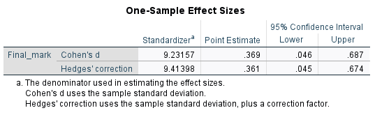
This tells us that our sample mean is \(0.369\) standard deviations from the test value, and indicates a small to medium effect (generally a Cohen’s \(d\) of magnitude \(0.2\) is considered small, \(0.5\) medium and \(0.8\) or above large).
Paired samples \(t\) test
A paired samples \(t\) test is used to test whether there is a significant difference between means for continuous variables for two related groups. For example, you would use it if you had a sample of individuals who had their heart rate recorded twice, before and after exercise, and you wanted to see if there was a significant difference between the two means. In this case the hypotheses (for a two-tailed hypothesis test) would be:
\(\textrm{H}_\textrm{0}\): There is no significant difference in heart rate before and after exercise
(\(\mu_{\textrm{HR before}} = \mu_{\textrm{HR after}}\), or \(\mu_{\textrm{HR before}} - \mu_{\textrm{HR after}} = 0\))
\(\textrm{H}_\textrm{A}\): There is a significant difference in heart rate before and after exercise
(\(\mu_{\textrm{HR before}} \neq \mu_{\textrm{HR after}}\), or \(\mu_{\textrm{HR before}} - \mu_{\textrm{HR after}} \neq 0\))
Before conducting a paired samples \(t\) test you need to check that the following assumptions are valid:
Assumption 1: The sample is a random sample that is representative of the population.
Assumption 2: The observations are independent, meaning that measurements for one subject have no bearing on any other subject’s measurements.
Assumption 3: Both variables as well as the difference variable (i.e. the differences between each data pair) are normally distributed, or the sample size is large enough that the sampling distribution of the mean approximates a normal distribution.
</div>
If the normality assumption is violated, or if you have ordinal variables rather than continuous ones (such as blood pressures recorded as low, normal or high), the Wilcoxon signed rank test should be used instead.
Assuming the assumptions for the paired samples \(t\) test are met though, and the test is conducted using statistical software (e.g. SPSS as in this example), the results should include the following statistics:


When analysing the results of the test, you should observe the descriptive statistics first in order to get an idea of what is happening in the sample. For example, the difference between the before and after sample means is \(48.70\) (this value can be calculated from the means in the first table, and is also displayed in the second table; the fact that it is negative simply indicates that the heart rate after is greater than the heart rate before). To test whether or not this difference is statistically significant requires the \(p\) value (which is listed as ‘Sig. (2-tailed)’ in the second table, as we have conducted a two-tailed hypothesis test) and the confidence interval for the difference. In terms of the \(p\) value, if we are assessing statistical significance at the \(.05\) level of significance then:
- If \(p \leqslant .05\) we reject \(\textrm{H}_\textrm{0}\) and conclude that the means of the two related groups are significantly different.
- If \(p > .05\) we do not reject \(\textrm{H}_\textrm{0}\) and conclude that the means of the two related groups are not significantly different.
In this case, our \(p\) value of \(< .001\) indicates that the difference between the means is statistically significant.
This is confirmed by the confidence interval of (\(-52.64574\), \(-44.75426\)) for the difference between the means. Because this confidence interval does not contain zero it again means the difference is statistically significant, and in fact, we are \(95\%\) confident that the population mean heart rate after exercise is between \(44.75426\) and \(52.64574\) bpm higher than the population mean heart rate before exercise.
Note that while the test statistic (\(t\)) and degrees of freedom (\(df\)) should both generally be reported as part of your results, you do not need to interpret these when assessing the significance of the difference.
If you would like to practise interpreting the results of a paired samples \(t\) test for statistical significance, have a go at one or both of the following activities.
To evaluate practical significance in situations where a paired samples \(t\) test is appropriate, Cohen’s \(d\) can again be used to measure the effect size. This time it measures how many standard deviations the two means are separated by, and should also be able to be obtained using statistical software. For example, the Cohen’s \(d\) for our heart rate data is included in the following output:
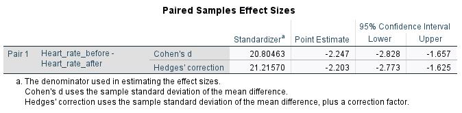
This tells us that our two sample means are separated by \(3.947\) standard deviations, and indicates a very large effect (generally a Cohen’s \(d\) of magnitude \(0.2\) is considered small, \(0.5\) medium and \(0.8\) or above large).
Independent samples \(t\) test
An independent samples \(t\) test is used to test whether there is a significant difference in means for a continuous variable for two independent groups. For example, you would use it if you collected data on hours spent watching TV each week and you wanted to see if there was a significant difference in the mean hours for males and females. In this case the hypotheses would be:
\(\textrm{H}_\textrm{0}\): There is no significant difference in TV hours per week for males and females
(\(\mu_{\textrm{males}} = \mu_{\textrm{females}}\), or \(\mu_{\textrm{males}} - \mu_{\textrm{females}} = 0\))
\(\textrm{H}_\textrm{A}\): There is a significant difference in TV hours per week for males and females
(\(\mu_{\textrm{males}} \neq \mu_{\textrm{females}}\), or \(\mu_{\textrm{males}} - \mu_{\textrm{females}} \neq 0\))
Before conducting an independent samples \(t\) test you need to check that the following assumptions are valid:
Assumption 1: The sample is a random sample that is representative of the population.
Assumption 2: The observations are independent, meaning that measurements for one subject have no bearing on any other subject’s measurements.
Assumption 3: The variable is normally distributed for both groups, or the sample size is large enough that the sampling distribution of the mean approximates a normal distribution.
</div>
If the normality assumption is violated, or if you have an ordinal variable rather than a continuous one (such as hours recorded in ranges), the Mann-Whitney U test should be used instead.
Assuming the assumptions for the independent samples \(t\) test are met though, and the test is conducted using statistical software (e.g. SPSS as in this example), the results should include the following statistics:
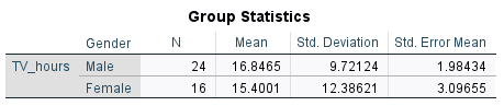

When analysing the results of the test, you should observe the descriptive statistics first in order to get an idea of what is happening in the sample. For example, the difference between the sample means for males and females is \(1.44641\) (this value can be calculated from the means in the first table, and is also displayed in the second table).
Next, note that there are actually five \(p\) values (and two confidence intervals) in the second table. Two are applicable when the variances of the two groups are approximately equal (those in the ‘One-sided p’ and ‘Two-Sided p’ columns in the top row of the table; we will interpret the ‘Two-Sided p’ value as we have conducted a two-tailed hypothesis test), two are applicable when the variances of the two groups are not approximately equal (those in the ‘One-sided p’ and ‘Two-Sided p’ columns in the bottom row of the table; we will interpret the ‘Two-Sided p’ value as we have conducted a two-tailed hypothesis test), and the remaining one (the first one in the table, in the ‘Sig.’ column) is used to determine which situation we have.
We need to interpret the latter first, which is the \(p\) value for Levene’s Test for Equality of Variances. The null hypothesis for this test is that the variances are equal, so if \(p \leqslant .05\) it is evidence to reject this null hypothesis and assume unequal variances, while if \(p > .05\) there is not enough evidence to reject the null hypothesis and equal variances can be assumed. Depending on which is which, determines which of the other \(p\) values (and confidence intervals) you should interpret. In this case, the \(p\) value of \(.257\) indicates we can assume equal variances, and that we should interpret the (two-sided) \(p\) value in the top row of the remainder of the table. Again, the interpretation of this \(p\) value is that:
- If \(p \leqslant .05\) we reject \(\textrm{H}_\textrm{0}\) and conclude that the means of the two groups are significantly different.
- If \(p > .05\) we do not reject \(\textrm{H}_\textrm{0}\) and conclude that the means of the two groups are not significantly different.
In this case, our \(p\) value of \(.682\) indicates that the difference between the means is not statistically significant.
This is confirmed by the confidence interval of (\(-5.64375\), \(8.53657\)) for the difference between the means. Because this confidence interval contains zero it again means the difference is not statistically significant, and in fact, we are \(95\%\) confident that the difference in mean hours spent watching TV each week for males and females is between \(-5.64375\) and \(8.53657\) hours.
Note that while the test statistic (\(t\)) and degrees of freedom (\(df\)) should both generally be reported as part of your results, you do not need to interpret these when assessing the significance of the difference.
If you would like to practise interpreting the results of an independent samples \(t\) test for statistical significance, have a go at one or both of the following activities.
To evaluate practical significance in situations where an independent samples \(t\) test is appropriate, Cohen’s \(d\) can again be used to measure the effect size. This time it measures how many standard deviations the two means are separated by, and should also be able to be obtained using statistical software. For example, the Cohen’s \(d\) for our TV hours data is included in the following output:
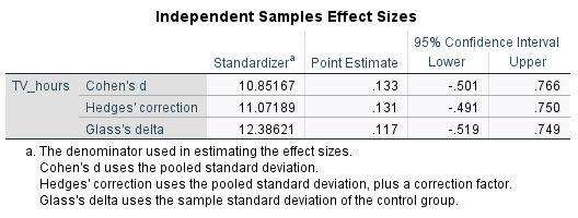
This tells us that our two sample means are separated by \(0.133\) standard deviations, and indicates a very small effect (generally a Cohen’s \(d\) of magnitude \(0.2\) is considered small, \(0.5\) medium and \(0.8\) or above large).
One-way ANOVA
One-way ANOVA is similar to the independent samples \(t\) test, but is used when three or more groups are compared. While one-way ANOVA is the only type of ANOVA covered here, note that it is just one in a family of ANOVA tests with other types including the following:
- Factorial ANOVA: used to test for differences in means between groups when there are two or more independent variables.
- One-way repeated measures ANOVA: used to test for differences in means between three or more related samples.
- ANCOVA (one-way analysis of covariance): used to test for differences between two or more independent samples after controlling for the effects of a third variable (covariate).
- MANOVA (multivariate analysis of variance): used to simultaneously test for differences between groups on multiple dependent variables.
Returning to the one-way ANOVA, consider that you have a data set containing the final marks of a sample of students studying one of three different units. You could use the one-way ANOVA to see if there is a significant difference in the mean marks for any of the units, in which case the hypotheses would be:
\(\textrm{H}_\textrm{0}\): There is no significant difference in the mean final mark for any of the three units.
(\(\mu_{\textrm{unit 1}} = \mu_{\textrm{unit 2}} = \mu_{\textrm{unit 3}}\))
\(\textrm{H}_\textrm{A}\): The mean final mark of at least one of the units is significantly different to the others.
Before conducting a one-way ANOVA you need to check that the following assumptions are valid:
Assumption 1: The sample is a random sample that is representative of the population.
Assumption 2: The observations are independent, meaning that measurements for one subject have no bearing on any other subject’s measurements.
Assumption 3: The variable is normally distributed for each of the groups, or the sample size is large enough that the sampling distribution of the mean approximates a normal distribution.
Assumption 4: The populations being compared have equal variances.
</div>
If the normality assumption is violated, or if you have an ordinal variable rather than a continuous one (such as final grade categories), the Kruskal-Wallis one-way ANOVA should be used instead. If the equal variances assumption is violated, you should use the Brown-Forsythe or Welch test instead.
Assuming the assumptions for the one-way ANOVA are met though, and the test is conducted using statistical software (e.g. SPSS as in this example), the results should include the following statistics:
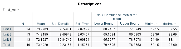
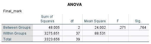
When analysing the results of the test, you should observe the descriptive statistics first in order to get an idea of what is happening in the sample. For example, the sample means are \(73.2203\) for Unit 1, \(74.8499\) for Unit 2 and \(72.1527\) for Unit 3. To test whether or not there are statistically significant differences between any of these three means requires the \(p\) value (which is listed as ‘Sig.’ in the second table), which we can interpret as follows:
- If \(p \leqslant .05\) we reject \(\textrm{H}_\textrm{0}\) and conclude that the mean of at least one of the groups is significantly different to the others.
- If \(p > .05\) we do not reject \(\textrm{H}_\textrm{0}\) and conclude that there are no significant differences between the means of any of the groups.
In this case, our \(p\) value of \(.764\) indicates that there are no significant differences in mean final grades between any of the units.
Note that while the test statistic (\(F\)) and degrees of freedom (\(df\)) should both generally be reported as part of your results, you do not need to interpret these when assessing the significance of the difference. Note also that if a one-way ANOVA is conducted and it turns out that at least one of the means is different, you will need to investigate further to determine where the difference lies using post hoc tests, for example Tukey’s HSD.
For now though, if you would like to practise interpreting the results of a one-way ANOVA for statistical significance, have a go at one or both of the following activities.
To evaluate practical significance in situations where a one-way ANOVA is appropriate, eta-squared can be used to measure the effect size. This indicates how much variability (as a percentage) in the dependent variable can be attributed to the independent variable, and should also be able to be obtained using statistical software. For example, the eta-squared for our final mark data is included in the following output:
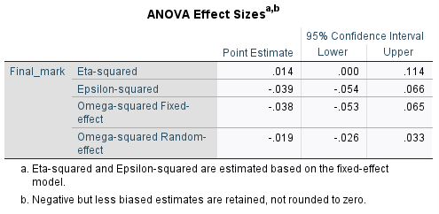
The eta-squared value of \(0.014\) tells us that \(1.4\%\) of the variability in the final marks can be attributed to the unit of study, which is a small effect (generally an eta-squared of \(0.01\) is considered small, \(0.059\) medium and \(0.138\) or above large).Assessing relationships
One of the reasons you may wish to do a hypothesis test is to determine whether there is a statistically significant relationship between two or more variables. Different tests are required for this based on the type of variables, and this page details two of the most common tests for assessing relationships between two variables.
In brief, it covers the following:
- When to conduct a Chi-square test of independence, and how to interpret the results
- When to conduct a test of Pearson’s correlation, and how to interpret the results
</div>
Chi-square test of independence
The chi-square test of independence is a non-parametric test used to determine whether there is a statistically significant association between two categorical variables. For example, it could be used to test whether there is a statistically significant association between employment status (full time or part time) and owning a pet. In this case the hypotheses would be:
\(\textrm{H}_\textrm{0}\): There is no association between employment status and owning a pet
\(\textrm{H}_\textrm{A}\): There is an association between employment status and owning a pet
Before conducting a chi-square test of independence you need to check that the following assumptions are valid:
Assumption 1: The categories used for the variables are mutually exclusive (i.e. people or things can’t fit into more than one category).
Assumption 2: The categories used for the variables are exhaustive (i.e. there is a category for everyone or everything).
Assumption 3: No more than \(20\%\) of the expected frequencies are less than \(5\) (if this is violated Fisher’s exact test can be used instead).
</div>
Note that these first two assumptions simply require appropriate categories for both of the variables, while information for the third assumption should be provided with the results of the test (i.e. the \(0.0\%\) below the second table that follows).
Assuming the assumptions for the chi-square test are met, and the test is conducted using statistical software (e.g. SPSS as in this example), the results should include the following statistics:
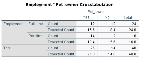
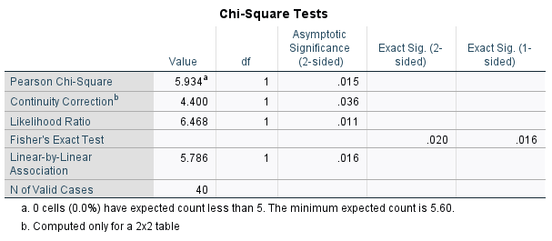
When analysing the results of the test, you should observe the descriptive statistics first in order to get an idea of what is happening in the sample. For example, the fact that there is a reasonably large difference between the Counts and Expected Counts in the cross-tabulation indicates that there is at least some association between the variables in the sample. To test whether or not this association is statistically significant requires the \(p\) value for Pearson’s chi-square test though, which is listed as ‘Asymptotic Significance (2-sided)’. If we are assessing statistical significance at the \(.05\) level of significance then:
- If \(p \leqslant .05\) we reject \(\textrm{H}_\textrm{0}\) and conclude that there is a statistically significant association between the variables.
- If \(p > .05\) we do not reject \(\textrm{H}_\textrm{0}\) and conclude that there is not a statistically significant association between the variables.
In this case, our \(p\) value of \(.015\) indicates that the association between between employment status and owning a pet is statistically significant.
Note that while the chi-square value and degrees of freedom (\(df\)) should both generally be reported as part of your results, you do not need to interpret these when assessing the significance of the difference.
If you would like to practise interpreting the results of a chi-square test for statistical significance, have a go at the following activity.
A few different statistics can be used to calculate effect size (and therefore evaluate practical significance) in situations where a chi-square test of independence has been conducted. Which statistic to use depends on a few different things, including the number of categories for each variable, the type of variables (nominal or ordinal) and the nature of the study. In the case where there are only two categories for each variable, effect size can be measured using phi (\(\phi\)) (note that an extension of phi for nominal variables with more than two categories is Cramer’s V, while other measures of effect size include relative risk and odds ratio). This should also be able to be obtained using statistical software, and for example phi for our employment and pet example is included in the following output:
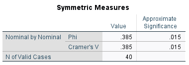
This is considered a medium to large effect (generally a phi of magnitude 0.1 is considered small, 0.3 medium and 0.5 or above large).
Pearson’s correlation
A hypothesis test of Pearson’s correlation coefficient is used to determine whether there is a statistically significant linear correlation between two continuous variables. For example, it could be used to test whether there is a statistically significant linear correlation between heart rates before and after exercise. In this case the hypotheses would be:
\(\textrm{H}_\textrm{0}\): There is no linear correlation between heart rates before and after exercise in the population
\(\textrm{H}_\textrm{A}\): There is linear correlation between heart rates before and after exercise in the population
Before conducing a hypothesis test of Pearson’s correlation coefficient you need to check that the following assumptions are valid:
Assumption 1: The observations are independent, meaning that measurements for one subject have no bearing on any other subject’s measurements.
Assumption 2: Both variables are normally distributed, or the sample size is large enough that the sampling distribution of the mean approximates a normal distribution.
Assumption 3: There is a linear relationship between the variables, as observed in the scatter plot (while Pearson’s correlation coefficient can still be calculated if there is not, this hypothesis test is not necessary or appropriate if the relationship is not linear).
Assumption 4: There is a homoscedastic relationship between the variables (i.e. variability in one variable is similar across all values of the other variable), as observed in the scatter plot (dots should be similar distance from the line of best fit all the way along).
</div>
If the variables are not normally distributed, or if the data is ordinal, you should use Spearman’s rho or Kendall’s tau-\(b\) instead.
Assuming the assumptions for Pearson’s correlation are met though, and the test is conducted using statistical software (e.g. SPSS as in this example), the results should include the following statistics:
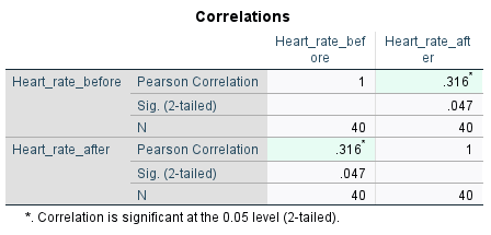
Included in the output is Pearson’s correlation (\(r\)) value (of \(.316\) in this case) which you should interpret first in order to get an idea of what is happening in the sample. For example, the fact that this \(r\) value is positive and relatively close to \(0\) indicates that there is a weak positive linear correlation between the variables in the sample. To test whether or not this linear correlation is statistically significant requires the \(p\) value though, which in the table is listed as ‘Sig. (2-tailed)’. If we are assessing statistical significance at the \(.05\) level of significance then:
- If \(p \leqslant .05\) we reject \(\textrm{H}_\textrm{0}\) and conclude that there is statistically significant linear correlation between the variables.
- If \(p > .05\) we do not reject \(\textrm{H}_\textrm{0}\) and conclude that there is not statistically significant linear correlation between the variables.
In this case, our \(p\) value of \(.047\) shows that the linear correlation between the before and after heart rates is statistically significant.
If you would like to practise interpreting the results of a Pearson’s correlation hypothesis test for statistical significance, have a go at the following activity.
Finally, note that the correlation coefficient is a measure of effect size, so a separate measure does not need to be calculated to interpret practical significance (again generally a value of magnitude \(0.1\) is considered small, \(0.3\) medium and \(0.5\) and above large).
Furthermore, the percentage of variation in the dependent variable that can be accounted for by variation in the independent variable can be found by calculating \(r^2\). This is known as the coefficient of determination.
In the previous heart rate example the effect size is medium (\(.316\)), and the coefficient of determination of \(.0999\) indicates that \(9.99\%\) of the variation in the after heart rate can be accounted for by variation in the before heart rate.
Regression analysis
Regression analysis is a statistical method used to model and explain the relationship between variables, and to make predictions about one variable based on one or more others. Different types of regression are required depending on the type of variables involved, and this page outlines two of the most common types.
In brief, it covers the following:
- When to use linear regression, and how to interpret the results
- When to use logistic regression, and how to interpret the results
</div>
Linear regression
Linear regression is used to model the relationship between one or more independent variables (which can be continuous or categorical) and a continuous dependent variable. It builds on the idea of correlation, as it also describes a linear relationship between variables, but it allows this relationship to be expressed as an equation that can be used to make predictions. Furthermore, while simple linear regression involves only one independent variable (as with correlation), most of the time there are actually multiple factors that may influence the outcome - and these can all be accounted for in multiple linear regression.
For example, multiple linear regression can be used to examine how factors such as heart rate before exercise, age and gender influence heart rate after exercise. It does this by providing information about how well the variables explain heart rate after exercise overall, as well as the effect of each variable individually while accounting for the other variables in the model.
Before conducting linear regression, you need to check that the following assumptions are valid:
Assumption 1: The observations are independent, meaning that measurements for one subject have no bearing on any other subject’s measurements.
Assumption 2: There is a linear relationship between each independent variable and the dependent variable. This can be assessed by examining scatter plots.
Assumption 3: There are no significant outliers that unduly influence the results.
Assumption 4: The independent variables are not too highly correlated with each other (multicollinearity), as this can make it difficult to determine how each variable is influencing the dependent variable.
Assumption 5: The residuals (differences between the observed and predicted values) are approximately normally distributed, and their variability is similar across all values of the predicted variable (homoscedasticity).
</div>
In adition, note that it is also important to have a sufficiently large sample size relative to the number of independent variables included in the regression model. A commonly used rule of thumb is to have around \(10–15\) cases for each independent variable.
Assuming the assumptions for linear regression are met, and the analysis is conducted using statistical software (e.g. SPSS as in this example), the results should include the following statistics:


The first of these output tables is the Model Summary, which includes \(R^2\) and adjusted \(R^2\) values. While these both provide an indication of how well the model explains the variation in the dependent variable, the adjusted \(R^2\) value takes into account the number of independent variables in the model and provides a more accurate estimate of how well the model would perform in the population, so is typically the one used. In this case, the adjusted \(R^2\) value of \(.131\) indicates that \(13.1\%\) of the variation in heart rate after exercise can be explained by the independent variables in the model (heart rate before exercise, age and gender).
The second output table is the ANOVA table, which includes the overall \(p\) value for the model. This is used to determine whether the model as a whole is statistically significant. In this case, the \(p\) value of \(.045\) indicates that the model is statistically significant at the \(.05\) level.
The final output table is the Coefficients table, which shows the effect of each independent variable on the dependent variable while accounting for the other variables in the model. It includes both unstandardised coefficients (\(B\)) and standardised coefficients (\(\beta\)), along with associated \(p\) values. While both types of coefficient provide information about the relationship between the independent and dependent variables, the unstandardised coefficients are typically used for interpretation, as they indicates the expected change in the dependent variable for a one-unit increase in the independent variable.
In this example, heart rate before exercise has a positive coefficient (\(B = 0.763\)) and is statistically significant (\(p = .020\)). This indicates that, after accounting for age and gender, heart rate after exercise is expected to increase by \(0.763\) beats per minute for each additional beat per minute in heart rate before exercise.
Age also has a positive coefficient (\(B = 0.217\)) but is not statistically significant (\(p = .346\)). This indicates that, after accounting for the other variables, heart rate after exercise is expected to increase by \(0.217\) beats per minute for each additional year of age, although there is insufficient evidence that this relationship exists in the population.
Gender also has a positive coefficient (\(B = 7.239\)) and is not statistically significant (\(p = .066\)). Given that gender is coded as \(1\) for male and \(2\) for female, this indicates that, after accounting for the other variables, heart rate after exercise is expected to be \(7.239\) beats per minute higher for females than males, although there is insufficient evidence that this relationship exists in the population.
Overall, while the model is statistically significant, heart rate before exercise appears to be the only independent variable with clear evidence of a relationship with heart rate after exercise once the effects of age and gender are taken into account.
Logistic regression
Logistic regression is used to model the relationship between one or more independent variables (which can be continuous or categorical) and a categorical dependent variable. Most commonly, the dependent variable has two categories (for example yes/no or pass/fail), although logistic regression can also be extended to outcomes with more than two categories. Like linear regression, logistic regression allows the effect of multiple independent variables on an outcome to be examined while accounting for the other variables in the model. However, rather than modelling a linear relationship, it models the probability of an outcome occurring.
For example, logistic regression can be used to examine how factors such as study time, attendance and gender influence whether a student passes or fails a unit. It does this by providing information about how well the variables explain pass status overall, as well as the effect of each variable individually while accounting for the other variables in the model.
Before conducting logistic regression, you need to check that the following assumptions are valid:
Assumption 1: The observations are independent, meaning that measurements for one subject have no bearing on any other subject’s measurements.
Assumption 2: There is a linear relationship between any continuous independent variables and the log odds of the dependent variable.
Assumption 3: There are no significant outliers that unduly influence the results.
Assumption 4: The independent variables are not too highly correlated with each other (multicollinearity), as this can make it difficult to determine how each variable is influencing the dependent variable.
</div>
In addition, note that it is also important to have a sufficiently large sample size relative to the number of independent variables included in the regression model. A commonly used rule of thumb for logistic regression is to have at least \(10\) outcome events for each independent variable.
Assuming the assumptions for logistic regression are met, and the analysis is conducted using statistical software (e.g. SPSS as in this example), the results should include the following statistics:


The first of these output tables is the Omnibus Tests of Model Coefficients table, which includes the overall \(p\) value for the model (given in the ‘Model’ row). This is used to determine whether the model as a whole is statistically significant. In this case, the \(p\) value is less than \(.001\), indicating that the model is statistically significant at the \(.05\) level.
The second output table is the Model Summary table, which includes pseudo \(R^2\) values (Cox & Snell and Nagelkerke \(R^2\)). While these both provide an indication of how well the model explains the variation in the dependent variable, the Nagelkerke \(R^2\) value is typically preferred, as it is scaled to range from \(0\) to \(1\) and therefore provides a more interpretable estimate. In this case, the Nagelkerke \(R^2\) value of \(.605\) indicates that the independent variables explain a substantial amount of the variation in pass status, although a proportion remains unexplained.
The final output table is the Variables in the Equation table, which shows the effect of each independent variable on the dependent variable while accounting for the other variables in the model. It includes the regression coefficients (\(B\)), their associated \(p\) values, and odds ratios (\(Exp(B)\)). While the regression coefficients are used to construct the model, the odds ratios are typically used for interpretation, as they indicate how the odds of the outcome change for a one-unit increase in the independent variable.
In this example, study time has an odds ratio of \(2.125\), but is not statistically significant (\(p=.661\)). This indicates that, after accounting for attendance and gender, each additional hour of study time is associated with approximately a doubling of the odds of passing the unit, although there is insufficient evidence that this relationship exists in the population.
Attendance has an odds ratio of \(1.066\), but is not statistically significant (\(p=.895\)). This indicates that, after accounting for the other variables,each additional percentage point in attendance is associated with a small increase in the odds of passing, although there is insufficient evidence that this relationship exists in the population.
Gender has an odds ratio of \(2.599\), but is also not statistically significant (\(p=.351\)). Given that gender is coded as \(1\) for male and \(2\) for female, this indicates that, after accounting for the other variables, females are predicted to have over twice the odds of passing than males, although there is insufficient evidence that this difference exists in the population.
Overall, while the model is statistically significant, there is insufficient evidence that any of the individual variables are significantly associated with pass status once the other variables are taken into account. Further resources & glossary
Further Resources
Congratulations on making it to the end of the module! We hope you found it a useful introduction to the world of statistics. If you are interested in learning more about statistics, and in particular finding out about other statistical tests, you may like to make use of one or more of the following resources:
- The Beginner’s Guide to Statistical Analysis
- Statistics by Jim
- Online Statistics Education: A Multimedia Course of Study
Glossary
The following is a glossary of statistical terms used throughout this module. For more information on any of the terms please click on the relevant link.
A C D E H I L M N O P Q R S T V
A
Alternative hypothesis
Also known as the research hypothesis, and denoted by \(\textrm{H}_\textrm{A}\), the alternative hypothesis always states the opposite of the null hypothesis; i.e. it states that there is a difference or relationship between variables in a population.
See Hypothesis testing, Null hypothesis, Variable.
C
Categorical data
Data which is grouped into categories, such as data for a ‘gender’ or ‘smoking status’ variable. Categorical data can be further classified as nominal or ordinal.
See Data, Nominal data, Ordinal data.
Chi-square test of independence
A non-parametric test used to determine whether there is a statistically significant association between two categorical variables. The chi-square value is represented by \(\chi^2\)
See Categorical data, Non-parametric test.
Cohen’s \(d\)
A measure of effect size which determines how many standard deviations two means are separated by. It is commonly used to evaluate practical significance for \(t\) tests and ANOVA.
See Effect size, \(t\) test, One-way ANOVA.
Confidence interval
A range of values that a population statistic (e.g. the population mean) is expected to lie between with a given level of certainty (known as the confidence coefficient). The confidence coefficient is typically \(95\%\), in which case it is referred to as a \(95\%\) confidence interval.
See Population.
Confounding variable
A variable that may have an influence on the dependent (outcome) variable.
See Variable.
Continuous data
Data which is measured on a continuous numerical scale and which can take on a large number of possible values, such as data for a ‘weight’ or ‘distance’ variable. Continuous data can be further classified as interval or ratio.
See Interval data, Ratio data, Variable.
Cross-tabulation (contingency table)
A table used to display information for two categorical variables. Categories of the independent variable are listed in the rows and categories of the dependent variable are listed in the columns, with each cell containing the frequency (number) of subjects that fall into that combination of categories. Percentages are often also included, along with totals.
See Categorical data, Dependent variable, Independent variable.
D
Data
Observations and measurements which have been collected in some way, often through research. Quantitative data measures quantities and is recorded as numbers, while qualitative data records qualities in terms of different categories or in terms of thoughts, feelings and opinions.
Discrete data
Data which measures counts or numbers of events, such as data for a ‘class attendance’ variable. It can be treated as either categorical or continuous, depending on how many values are possible.
See Data.
Degrees of freedom
The number of values that are free to vary when calculating an estimate. This is commonly reported as part of the results of various hypothesis tests.
See Hypothesis testing.
Dependent variable (outcome variable)
When testing for a relationship between pairs of variables, the dependent variable is the one that is potentially influenced, affected or predicted by the other variable.
See Variable.
Descriptive statistics
Statistics that are used to summarise and describe a variable or variables for a sample of data.
See Data, Sample, Variable.
E
Effect size
Effect size measures the magnitude of a difference or relationship between variables. It is used to provide evidence of whether it is meaningful in real life (i.e. has practical significance), and is calculated differently for different statistical tests.
See Cohen’s \(d\), Odds ratio, Practical significance, Variable.
H
Hypothesis testing
Hypothesis testing is used to determine whether a difference or relationship observed in a sample is statistically significant in terms of the population from which the sample was drawn. This can be assessed by interpreting the resulting \(p\) value.
See Alternative hypothesis, Null hypothesis, \(p\) value, Population, Sample, Statistical significance.
I
Independent samples \(t\) test
A parametric inferential statistical test used to determine whether there is a statistically significant difference between the mean of a continuous variable for two independent (unrelated) groups.
See Continuous data, Inferential statistics, Mean, Parametric test, Statistical significance.
Independent variable (predictor or exposure variable)
When testing for a relationship between pairs of variables, the independent variable is the one that potentially influences, affects or predicts the other variable.
See Variable.
Inferential statistics
Statistics that are used to draw inferences about the wider population from which a sample of data was drawn.
See Population, Sample.
Interquartile range
The interquartile range is a measure of dispersion appropriate in situations where the median is used as the measure of central tendency. It is calculating by finding the difference between the first and third quartiles.
See Measure of central tendency, Measure of dispersion, Median, Quartiles.
Interval data
Continuous data that does not have an absolute zero, and where negative numbers also have meaning, such as for a ‘temperature in degrees Celsius variable’.
See Continuous data.
L
Level of significance
In a hypothesis test, the level of significance (denoted by \(\alpha\)) determines exactly how small the \(p\) value can be before the null hypothesis is rejected. It is typically \(5\%\) (\(.05\))
See Hypothesis testing, Null hypothesis, \(p\) value
M
Mean
The mean is the arithmetic average of a data set, calculated by adding all of the data together and dividing through by the total number of values. It is the most commonly used measure of central tendency. The sample standard deviation is denoted by \(\bar{x}\), while the population mean is denoted by \(\mu\).
See Measure of central tendency, Population, Sample.
Measure of central tendency
A descriptive statistic which summarises a continuous variable by finding the average, central or typical member. Examples of measures of central tendency are the mean, median and mode.
See Continuous data, Descriptive statistic, Mean, Median, Mode.
Measure of dispersion
A descriptive statistic which summarises a continuous variable by finding out how widely it is spread or dispersed. Examples of measures of dispersion are the range, interquartile range, variance and standard deviation.
See Continuous data, Descriptive statistic, Interquartile range, Range, Standard deviation, Variance.
Median
The median is a more appropriate measure of central tendency than the mean when the data is affected by outliers or is skewed. It is calculated by finding the middle value (or average of two middle values) when the data set is sorted from smallest to largest.
See Mean, Measure of central tendency, Outlier, Skewness.
Mode
The mode is the most frequently occurring value (or values) in the data set; it is a less commonly used measure of central tendency.
See Measure of central tendency.
N
Nominal data
Categorical data where the categories do not have an order, such as for a ‘marital status’ variable. If there are only two categories, then the terms binary and/or dichotomous are often also used.
See Categorical data.
Non-parametric test
An inferential statistical test that doesn’t require the variable(s) to be normally distributed, and doesn’t require continuous data.
See Continuous data, Inferential statistics, Normal distribution.
Normal distribution
A distribution (spread) of data that has two key properties:
1. The mean, median and mode are all equal.
2. Fixed proportions of the data lie within certain numbers of standard deviations from the mean (\(68\%\) within one standard deviation, \(95\%\) within two standard deviations and \(99.7\%\) within three standard deviations).
See Data, Mean, Median, Mode, Standard deviation.
Null hypothesis
Denoted by \(\textrm{H}_\textrm{0}\), the null hypothesis always states that there is no difference or relationship between variables in a population.
See Alternative hypothesis, Hypothesis testing, Variable.
O
Odds ratio
A measure of effect size used when testing for association between an exposure and an outcome (e.g. using a Chi-square test), an odds ratio compares the odds of exposure in the group with the outcome to the odds of exposure in the group without the outcome. An odds ratio of \(1\) indicates no difference between the two groups, while an odds ratio greater than \(1\) indicates that the group with the outcome are more likely to have had the exposure, and an odds ratio less than \(1\) indicates that the group with the outcome are less likely to have had the exposure.
See Chi-square test of independence.
One sample \(t\) test
A parametric inferential statistical test used to determine whether there is a statistically significant difference between the mean of a continuous variable and a test value (some hypothesised value).
See Continuous data, Inferential statistics, Mean, Parametric test, Statistical significance.
One-way ANOVA (analysis of variance)
A parametric inferential statistical test used to determine whether there are any statistically significant differences between the means of a continuous variable for three or more independent (unrelated) groups.
See Continuous data, Inferential statistics, Mean, Parametric test, Statistical significance.
Ordinal data
Categorical data where the categories do have an order, such as for a ‘satisfaction level’ variable.
See Categorical data.
Outlier
An outlier is any data point that lies well above or below the other data; in particular, over \(1.5\) interquartile ranges below the first quartile or \(1.5\) interquartile ranges above the third quartile.
See Interquartile range, Quartiles.
P
\(p\) value
The \(p\) value for a hypothesis test is the probability of obtaining a given test statistic if the null hypothesis is true. A small \(p\) value indicates a low probability, and in particular if the \(p\) value is less than the level of significance it provides evidence to reject the null hypothesis (and hence of statistical significance).
See Hypothesis test, Level of significance, Null hypothesis, Statistical significance, Test statistic.
Paired samples \(t\) test
A parametric inferential statistical test used to determine whether there is a statistically significant difference between the means of continuous variables for two related groups.
See Continuous data, Inferential statistics, Mean, Parametric test, Statistical significance.
Parametric test
An inferential statistical test that requires at least one continuous variable, and which requires continuous variables to be normally distributed (or the sample size to be large enough that the sampling distribution of the mean approximates a normal distribution).
See Continuous data, Inferential statistics, Normal distribution.
Pearson’s correlation coefficient
Pearson’s correlation coefficient, denoted by \(r\), is used to determine whether there is a linear correlation (straight line relationship) between two continuous variables. It can range from \(-1\) to \(1\), with values close to \(-1\) indicating strong negative correlation, values close to \(1\) indicating strong positive correlation, and values close to \(0\) indicating no correlation.
See Continuous data.
Percentiles
A measure of dispersion that measures position from the beginning of an ordered data set, and can be used to measure the relative standing of a particular data point.
See Measure of dispersion.
Population
A population is every member of a group of interest. Normally it is not possible or feasible to collect data from the entire population, so a random sample is used instead to draw inferences about the population.
See Data, Inferential statistics, Sample.
Power
The power of a hypothesis test is the probability that the test will find an effect if one actually exists; in other words, that an incorrect null hypothesis will in fact be rejected.
See Hypothesis test, Null hypothesis.
Practical significance
Practical significance refers to whether or not a difference or relationship between variables is meaningful in a practical sense (i.e. in real life). It is determined by calculating an effect size.
See Effect size, Variable.
Q
Quartiles
A specific type of percentiles which divide the data set into quarters. In particular, the \(25\)th percentile is known as the first or lower quartile, the \(50\)th percentile is known as the median, and the \(75\)th percentile is known as the third or upper quartile.
See Median, Percentiles
R
Range
The simplest measure of dispersion, the range is the difference between the smallest and largest value in a data set.
See Measure of dispersion.
Ratio data
Continuous data that does have an absolute zero, and where negative numbers do not have meaning, such as for a ‘height’ variable.
See Continuous data.
S
Sample
A sample is a subset of a population. It can be analysed using descriptive statistics, or used to draw inferences about the wider population using inferential statistics.
See Descriptive statistics, Inferential statistics, Population.
Standard deviation
Standard deviation is the most commonly used measure of dispersion, appropriate in situations where the mean is used as the measure of central tendency. It is the square root of the variance, and measures how much deviation there is from the mean. Sample standard deviation is denoted by \(s\), while population standard deviation is denoted by \(\sigma\)
See Mean, Measure of central tendency, Measure of dispersion, Population, Sample, Variance.
Statistical significance
Statistical significance refers to whether or not a difference or relationship between variables observed in a sample could have occurred due to random chance alone. It is determined by conducting a hypothesis test.
See Hypothesis test, Sample, Variable.
T
Test statistic
A value calculated as the result of a hypothesis test, the test statistic compares the value of the sample statistic (for example, the sample mean) with the value specified by the null hypothesis for the population statistic.
See Hypothesis testing, Mean, Null hypothesis, Population, Sample.
V
Variable
A characteristic or attribute that you are observing, measuring and recording data for, e.g height, weight, eye colour, dog breed, etc.
See Data.
Variance
A measure of dispersion that measures how much deviation there is from the mean, the square root is usually taken in order to find the standard deviation.
See Mean, Measure of dispersion, Standard deviation.
Feedback
If you would like to provide feedback on this module please do so by answering some or all of the questions in the form below. Alternatively for any questions about the module please contact Library-UniSkills@curtin.edu.au
We review this feedback regularly, and take your suggestions on board to improve the module. Thank you for your feedback!
Explore more here
About UniSkills
UniSkills was created and is maintained by Curtin University Library. To report issues with UniSkills contact Library Help.
Twemoji icons by Twitter, Inc and other contributors, licensed under a CC-BY 4.0 licence.
Except where otherwise noted, UniSkills content in all it’s forms (website, PDFs etc) are licensed under a Creative Commons Attribution ShareAlike 4.0 International Licence. We ask that you attribute any use of the content as created by Curtin University Library with a link to the Library website.
This license does not extend to other Curtin University and Curtin University Library webpages, or to Curtin branding and trademarks. Curtin University’s copyright information is available on the Curtin website.