Introduction to statistics
One of the reasons you may wish to do a hypothesis test is to determine whether there is a statistically significant relationship between two or more variables. Different tests are required for this based on the type of variables, and this page details two of the most common tests for assessing relationships between two variables.
Chi-square test of independence
The chi-square test of independence is a non-parametric test used to determine whether there is a statistically significant association between two categorical variables. For example, it could be used to test whether there is a statistically significant association between employment status (full time or part time) and owning a pet. In this case the hypotheses would be:
\(\textrm{H}_\textrm{0}\): There is no association between employment status and owning a pet
\(\textrm{H}_\textrm{A}\): There is an association between employment status and owning a pet
Before conducting a chi-square test of independence you need to check that the following assumptions are valid:
Assumption 1: The categories used for the variables are mutually exclusive (i.e. people or things can’t fit into more than one category).
Assumption 2: The categories used for the variables are exhaustive (i.e. there is a category for everyone or everything).
Assumption 3: No more than \(20\%\) of the expected frequencies are less than \(5\) (if this is violated Fisher’s exact test can be used instead).
Note that these first two assumptions simply require appropriate categories for both of the variables, while information for the third assumption should be provided with the results of the test (i.e. the \(0.0\%\) below the second table that follows).
Assuming the assumptions for the chi-square test are met, and the test is conducted using statistical software (e.g. SPSS as in this example), the results should include the following statistics:
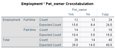
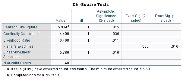
When analysing the results of the test, you should observe the descriptive statistics first in order to get an idea of what is happening in the sample. For example, the fact that there is a reasonably large difference between the Counts and Expected Counts in the cross-tabulation indicates that there is at least some association between the variables in the sample. To test whether or not this association is statistically significant requires the \(p\) value for Pearson’s chi-square test though, which is listed as ‘Asymptotic Significance (2-sided)’. If we are assessing statistical significance at the \(.05\) level of significance then:
- If \(p \leqslant .05\) we reject \(\textrm{H}_\textrm{0}\) and conclude that there is a statistically significant association between the variables.
- If \(p > .05\) we do not reject \(\textrm{H}_\textrm{0}\) and conclude that there is not a statistically significant association between the variables.
In this case, our \(p\) value of \(.015\) indicates that the association between between employment status and owning a pet is statistically significant.
Note that while the chi-square value and degrees of freedom (\(df\)) should both generally be reported as part of your results, you do not need to interpret these when assessing the significance of the difference.
If you would like to practise interpreting the results of a chi-square test for statistical significance, have a go at the following activity.
Activity
A few different statistics can be used to calculate effect size (and therefore evaluate practical significance) in situations where a chi-square test of independence has been conducted. Which statistic to use depends on a few different things, including the number of categories for each variable, the type of variables (nominal or ordinal) and the nature of the study. In the case where there are only two categories for each variable, effect size can be measured using phi (\(\phi\)) (note that an extension of phi for nominal variables with more than two categories is Cramer’s V, while other measures of effect size include relative risk and odds ratio). This should also be able to be obtained using statistical software, and for example phi for our employment and pet example is included in the following output:
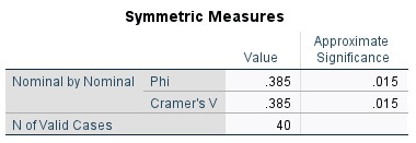
This is considered a medium to large effect (generally a phi of magnitude 0.1 is considered small, 0.3 medium and 0.5 or above large).
Pearson’s correlation
A hypothesis test of Pearson’s correlation coefficient is used to determine whether there is a statistically significant linear correlation between two continuous variables. For example, it could be used to test whether there is a statistically significant linear correlation between heart rates before and after exercise. In this case the hypotheses would be:
\(\textrm{H}_\textrm{0}\): There is no linear correlation between heart rates before and after exercise in the population
\(\textrm{H}_\textrm{A}\): There is linear correlation between heart rates before and after exercise in the population
Before conducing a hypothesis test of Pearson’s correlation coefficient you need to check that the following assumptions are valid:
Assumption 1: The observations are independent, meaning that measurements for one subject have no bearing on any other subject’s measurements.
Assumption 2: Both variables are normally distributed, or the sample size is large enough that the sampling distribution of the mean approximates a normal distribution.
Assumption 3: There is a linear relationship between the variables, as observed in the scatter plot (while Pearson’s correlation coefficient can still be calculated if there is not, this hypothesis test is not necessary or appropriate if the relationship is not linear).
Assumption 4: There is a homoscedastic relationship between the variables (i.e. variability in one variable is similar across all values of the other variable), as observed in the scatter plot (dots should be similar distance from the line of best fit all the way along).
If the variables are not normally distributed, or if the data is ordinal, you should use Spearman’s rho or Kendall’s tau-\(b\) instead.
Assuming the assumptions for Pearson’s correlation are met though, and the test is conducted using statistical software (e.g. SPSS as in this example), the results should include the following statistics:
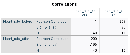
Included in the output is Pearson’s correlation (\(r\)) value (of \(-.209\) in this case) which you should interpret first in order to get an idea of what is happening in the sample. For example, the fact that this \(r\) value is negative and relatively close to \(0\) indicates that there is a weak negative linear correlation between the variables in the sample. To test whether or not this linear correlation is statistically significant requires the \(p\) value though, which in the table is listed as ‘Sig. (2-tailed)’. If we are assessing statistical significance at the \(.05\) level of significance then:
- If \(p \leqslant .05\) we reject \(\textrm{H}_\textrm{0}\) and conclude that there is statistically significant linear correlation between the variables.
- If \(p > .05\) we do not reject \(\textrm{H}_\textrm{0}\) and conclude that there is not statistically significant linear correlation between the variables.
In this case, our \(p\) value of \(.195\) shows that the linear correlation between the before and after heart rates is not statistically significant.
If you would like to practise interpreting the results of a Pearson’s correlation hypothesis test for statistical significance, have a go at the following activity.
Activity
Finally, note that the correlation coefficient is a measure of effect size, so a separate measure does not need to be calculated to interpret practical significance (again generally a value of magnitude \(0.1\) is considered small, \(0.3\) medium and \(0.5\) and above large).
Furthermore, the percentage of variation in the dependent variable that can be accounted for by variation in the independent variable can be found by calculating \(r^2\). This is known as the coefficient of determination.
In the previous heart rate example the effect size is small to medium (\(.209\)), and the coefficient of determination of \(.0437\) indicates that \(4.37\%\) of the variation in the after heart rate can be accounted for by variation in the before heart rate.