Introduction to statistics

Even if you are not carrying out statistical analysis yourself, it is important to be able to interpret and critically evaluate statistics that have been published as this will help you get the most out of journal articles and other academic sources that you read. This page explains some commonly reported statistics and how to interpret them.

Note that if you would like extra support with interpreting graphs and tables, or with performing key calculations, you may find the Statistics and probability page of the Numeracy fundamentals module useful. If you would like to carry out your own statistical analysis, information on how to do this is provided in later pages of this module.

Interpreting descriptive statistics

Descriptive statistics are used to summarise and describe the data you have collected. This may be:

• data for the whole population of interest (for example, everyone who attends a particular school), or
• data collected from a random sample of a larger population (for example, a random sample of people who were patients at a particular hospital over a two-year period).

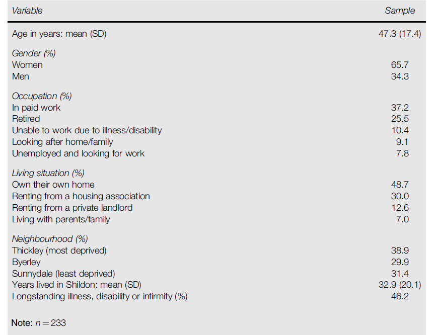
The key difference is that when you use data from a sample (which is most common), descriptive statistics cannot be used to draw conclusions about the wider population. For this reason, they are usually used together with other types of statistics. These will be explained shortly, but first we will look at the descriptive statistics in Table 1.

Table 1
Participant Characteristics

From “Examining Associations between Health, Wellbeing and Social Capital: Findings from a Survey Developed and Conducted using Participatory Action Research,” by S. Visram, S. Smith, N. Connor, G. Greig, & C. Scorer, 2018, Journal of Public Mental Health , 17 (3), p. 127 (https://doi.org/10.1108/JPMH-09-2017-0035). Copyright 2018 by Emerald Publishing Limited.

This data was collected from a sample of people who live in a particular city. The sample size is \(233\) (as shown by the \(n = 233\) at the bottom of the table), and there are two types of variables summarised:

1. categorical variables, which group data into categories (for example, the ‘Gender’ variable), and
2. continuous variables, which involve numerical data (for example, the ‘Age in years’ variable).

These two types of variables need to be analysed in different ways, and this has been done in the table. Let’s look at the categorical variables first.

Interpreting descriptive statistics for categorical variables

The categorical variables in this example have been summarised using percentages, which show the percentage of the sample that falls into each category for a variable. For example, the descriptive statistics for the ‘Gender’ variable show that \(65.7\%\) of the sample in Table 1 are women and \(34.3\%\) are men. Note that sometimes frequencies are used instead of percentages, and these show how many observations are in each category instead.

If you would like to learn more about descriptive statistics for categorical variables, including how to calculate them, please refer to the Descriptive statistics for one categorical variable section of this module. Alternatively, to practise interpreting descriptive statistics for categorical variables, try the following question.

Interpreting descriptive statistics for continuous variables

In this example, the continuous variables are summarised using two measures. The first measure is the mean, also called the arithmetic average. This is the most commonly used measure of central tendency, and is a single value that shows the central value of the data set. For example, in Table 1 the mean for the ‘Age in years’ variable is \(47.3\), which shows that the average (or central) age of the sample of \(233\) people is \(47.3\). The second measure is the standard deviation (SD), which is the most commonly used measure of dispersion. It is a single value that shows how varied (or spread out) the data is. In Table 1, the standard deviation for the ‘Age in years’ variable is \(17.4\). This is quite large compared to the mean, which shows that the ages in the sample of \(233\) people vary quite a lot.

Using both a measure of central tendency and a measure of dispersion gives a better summary of a continuous variable, as one measure on its own does not fully describe the data. For example, if we only knew that the mean age was \(47.3\), we would not know if all values were close to \(47.3\) or spread out across a wide range. Similarly, if we only knew that the standard deviation was \(17.4\), we would not know the central value of the data.

It is also important to understand that the mean and standard deviation are not always the best measures to use, as in some situations they do not describe the data accurately. This happens when:

• the data is skewed (not normally distributed, which will be explained later), or
• there are outliers (values that are much higher or lower than most of the data).

For example, suppose most people in Table 1 are aged between \(40\) and \(45\), but a small number are in their \(80\)s. These higher values would be outliers, and would increase the mean so it would no longer represent the central value accurately.

In these situations, the median is a more suitable measure of central tendency because it is not affected by outliers or skew, and the interquartile range is then used as the matching measure of dispersion. So when a variable is skewed or contains outliers, good research will use the median and interquartile range instead of the mean and standard deviation.

If you would like to learn more about descriptive statistics for continuous variables, including how to calculate them, refer to the Descriptive statistics for one continuous variable section of this module. Alternatively, to practise interpreting descriptive statistics for continuous variables, try the following question.

Interpreting inferential statistics

Inferential statistics are used to draw inferences about a wider population when data has been collected from a sample, rather than the whole population. This is usually necessary because collecting data from an entire population is often not practical. There are many different inferential statistical tests, used for different types of analysis and different types of variables. For example, different tests are used for continuous and categorical variables, and different tests may also be used for continuous variables depending on the sample size or the distribution (the pattern or spread of the data).

One type of distribution that can affect the choice of test is the normal distribution, which is a special type of distribution that large sets of naturally occurring continuous data often follow. It has two key properties:

• The mean, median and mode are all equal.
• Fixed proportions of the data fall within certain numbers of standard deviations from the mean (\(68\%\) within one SD, \(95\%\) within two SDs and \(99.7\%\) within three SDs).

When the sample size is small (typically fewer than about \(30\)), and sometimes even when it is larger, researchers may check whether continuous variables follow a normal distribution. This is not always reported in journal articles, but when it is, the Shapiro–Wilk test is often used to assess normality.

If an article states that variables pass this test (that is, the \(p\) value for the test is above \(.05\)), it means that normality can be assumed. For example, Power et al. (2019) refer to this when they state that their “outcomes were assessed for normality using Shapiro-Wilk” (p. 5).

In some cases, an article may state that variables have been transformed (for example, using a natural logarithm). This means the data was not originally normally distributed, but a mathematical change has been applied to make it follow a normal distribution. If you would like more information about the normal distribution and how to assess it, refer to The normal distribution page of this module.

If continuous variables are normally distributed, or can be transformed to be normally distributed, or if the sample size is large enough that this is not an issue, parametric tests are used. If the sample size is small and the variables are not normally distributed, or if the variables are categorical, nonparametric tests are used instead. Examples of parametric tests include \(t\) tests, ANOVA and Pearson’s correlation, while examples of nonparametric tests include chi-square tests, the Mann-Whitney U Test, the Wilcoxon Signed Rank Test, the Kruskal-Wallis One-Way ANOVA and Spearman’s rho.

For each of these tests, a good research article should report statistics that show whether any differences or relationships between variables are statistically significant and/or practically significant for the population. These terms, the relevant statistics, and how to interpret them are explained below. Alternatively, for more information on inferential statistics, including how to calculate statistical and practical significance, refer to the Inferential statistics page of this module.

Interpreting statistical significance

Statistical significance refers to how likely it is that what has been observed in a sample (for example, a difference in means or a relationship between variables) could have happened by random chance alone. If it is very unlikely that the result is due to chance, it is considered statistically significant in the population. To measure this, we use the \(p\) value.

The \(p\) value is the probability that the result occurred due to random chance. The smaller the \(p\) value, the less likely it is that the result is due to chance. To decide whether a \(p\) value is small enough, researchers use a level of significance, written as \(\alpha\). Different studies may use different levels, but a common value is \(.05\). In this case, a \(p\) value less than or equal to \(.05\) means that the result is considered statistically significant. Other common levels of significance used are \(.01\) and \(.001\), and articles may report the level at which results are significant (for example, significant at the \(.05\) or \(.01\) level).

Articles often include confidence intervals as well as \(p\) values. These are ranges of values that a population value is expected to fall within, with a certain level of confidence. This is usually \(95\%\), and is called a \(95\%\) confidence interval. Confidence intervals can also be used to assess statistical significance (at the \(.05\) level for a \(95\%\) confidence interval). In addition, they provide extra information such as the size and direction of a difference.

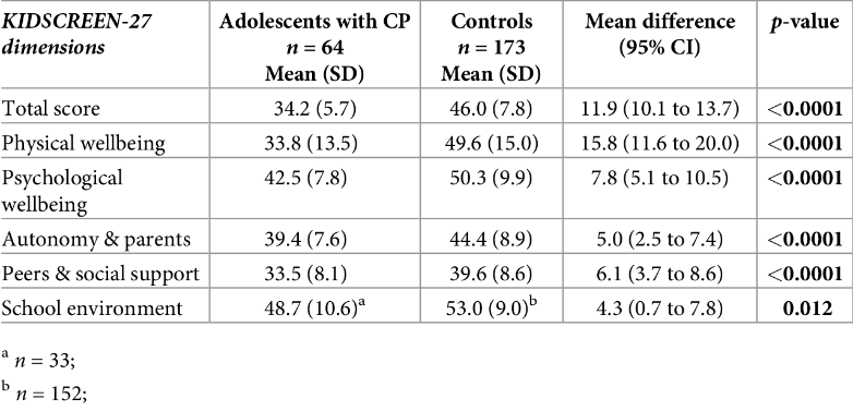
Table 2 shows descriptive statistics along with \(p\) values and confidence intervals for a set of variables. These statistics allow us to decide whether there is a statistically significant difference in means between two groups (adolescents with and without cerebral palsy) at the \(.05\) level of significance.

Table 2
Descriptive statistics, \(95\%\) CIs and \(p\) values for a study investigating mental and physical health of adults with cerebral palsy

From “Health-Related Quality of Life and Mental Health of Adolescents with Cerebral Palsy in Rural Bangladesh,” by R. Power, M. Muhit, E. Heanoy, T. Karim, N. Badawi, R. Akhter, & G. Khandaker, 2019, PLOS One , 14 (6), p. 9 (https://doi.org/10.1371/journal.pone.0217675). CC-BY.

Consider the ‘Total score’ variable, which measures overall health-related quality of life. The mean difference of \(11.9\) shows the difference between the two groups in the sample and is a descriptive statistic. The \(95\%\) confidence interval from \(10.1\) to \(13.7\) shows that we are \(95\%\) confident that the true difference in the population lies within this range, and because this interval does not include \(0\) (which would mean no difference), the result is significant at the \(.05\) level.

This result is also supported by the \(p\) value, as the fact that \(p < .0001\) shows that the result is statistically significant, not only at the \(.05\) level but even at the \(.0001\) level. The other variables in the table can be interpreted in the same way. To practise doing this, have a go at the following questions.

Interpreting practical significance

Practical significance refers to whether a result observed in a sample (for example, a difference in means or a relationship between variables) is meaningful in a real-life context. It is measured using an effect size, which is different for different statistical tests. For example:

• Cohen’s \(d\) is used with \(t\) tests
• Pearson’s correlation coefficient is used with Pearson’s correlation
• Phi, Cramer’s V, odds ratio and relative risk are commonly used with the chi-square test of independence.

Including practical significance in research provides important additional information, as statistical significance alone does not show whether a result is meaningful in practice because it is affected by sample size:

• In very large samples, very small differences that are not meaningful in real life can still be statistically significant.
• In very small samples, large and meaningful differences may not be statistically significant.

This idea is related to statistical power, which is the probability that a test will detect an effect of a certain size as statistically significant. Researchers can calculate how large a sample needs to be to detect an effect of a certain size at a chosen level of significance, for a given level of power (usually \(0.8\) or higher). For this reason, research articles may also report the power of a test.

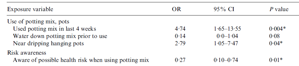
Returning to measures of effect size, and Table 3 presents odds ratios along with \(95\%\) confidence intervals and \(p\) values. The confidence intervals and \(p\) values show the statistical significance of the relationship between each exposure variable and the outcome variable (L.longbeachae infection), while the odds ratios show the practical significance of these relationships.

Table 3
Odds ratios, \(95\%\) CIs and \(p\) values for a study investigating L.longbeachae infection exposures involving potting mix

From “Does using Potting Mix make you Sick? Results from a Legionella Longbeachae Case-Control Study in South Australia,” by B. A. O’Connor, J. Carman, K. Eckert, G. Tucker, R. Givney, & S. Cameron, 2007, Epidemiology and Infection , 135 (1), p. 36 (https://doi.org/10.1017/S095026880600656X). Copyright 2006 by Cambridge University Press.

For each exposure variable, the odds ratio compares the odds of exposure in the group with L. longbeachae infection and the odds of exposure in the group without the infection. In other words, the odds ratio shows how many times more or less likely the group with the infection is to have the exposure compared to the group without the infection.

• An odds ratio less than \(1\) means the infected group is less likely to have the exposure.
• An odds ratio equal to \(1\) means both groups are equally likely to have the exposure.
• An odds ratio greater than \(1\) means the infected group is more likely to have the exposure.

For example, consider the first odds ratio which has a value of \(4.74\). This shows that people with L.longbeachae were \(4.74\) times more likely to have used potting mix in the last four weeks than those without the infection. Based on common guidelines for interpreting effect size, this represents a medium to large effect. (However, practical significance should always be interpreted in context, rather than relying only on cut-off values.)

Furthermore, the \(95\%\) confidence interval for this result is \(1.65\) to \(13.55\). This means we are \(95\%\) confident that the true value in the population lies within this range. Because this range does not include \(1\) (which would mean equal odds), the result is statistically significant at the \(.05\) level. This is also supported by the \(p\) value of \(.004\).

Research articles may also report adjusted odds ratios. These take into account other variables (called confounding variables) that may affect the outcome. Adjusted odds ratios are interpreted in the same way as the odds ratios described above.

If you would like to practise interpreting some of the other odds ratios in the table, have a go at the following questions.

Further example: interpreting one-way ANOVA

As another example of interpreting statistical and practical significance, consider Tables 4 and 5. These show the results of two one-way ANOVAs, which test for differences in mean ‘school attachment scores’:

• between students of different ages, and
• between students of different socio-economic groups.

Table 4
Descriptive statistics and one-way ANOVA statistics for a study investigating differences in school attachment scores between age groups

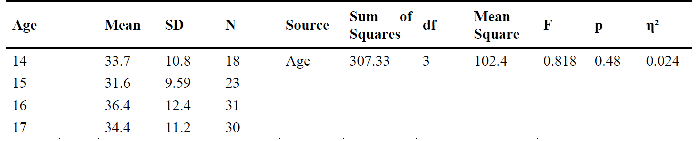
Table 5
Descriptive statistics and one-way ANOVA statistics for a study investigating differences in school attachment scores between socio-economic groups

From “School Attachment and Video Game Addiction of Adolescents with Divorced vs. Married Parents,” by B. TAS, 2019, TOJET: The Turkish Online Journal of Educational Technology , 18 (2), pp. 99-100 (https://files.eric.ed.gov/fulltext/EJ1211160.pdf). Copyright 2019 by The Turkish Online Journal of Educational Technology.

The \(p\) value in each table shows whether there is a statistically significant difference between the group means. If \(p\) is less than or equal to the level of significance, there is a statistically significant difference between the means of at least two groups. If \(p\) is greater than the level of significance, there is no statistically significant difference between any of the group means.

If a one-way ANOVA is statistically significant, more information is needed to identify which groups are different from each other. This information is usually provided through planned comparisons or post hoc tests. These produce additional \(p\) values, which are interpreted in the same way.

The tables also include an \(F\) value, which is the test statistic for a one-way ANOVA. Other statistical tests also have test statistics (for example, a \(t\) value for a \(t\) test or a chi-square value for a chi-square test). The \(F\) value compares the variability between groups and the variability within each group, and is calculated as a ratio of these two types of variability.

For example, an \(F\) value of \(0.818\) for the ‘Age’ variable means that the variability in school attachment scores between the four age groups is \(0.818\) times the variability within the groups. This shows that the variability between groups is smaller than the variability within groups. In general, the larger the \(F\) value (especially when it is greater than \(1\)), the more likely it is that there is a difference between the group means. However, the \(p\) value must be used to decide whether this difference is statistically significant.

Lastly, the tables also report eta-squared (\(\eta^2\)), which is a measure of effect size. Eta-squared shows the percentage of variability in the outcome (school attachment scores) that is explained by the variable (for example, age or socio-economic group). For example, the \(\eta^2\) value of \(0.024\) means that \(2.4\%\) of the variability in school attachment scores is explained by age. Guidelines suggested by Cohen (1988) state that \(.01\) is a small effect, \(.059\) is a medium effect and \(.138\) is a large effect.

Use the information above to answer the following questions:

References

Cohen, J. (1988). Statistical power analysis for the behavioral sciences (2nd ed.). Lawrence Erlbaum Associates, Inc.

Connor, B.A., Carman, J., Eckert, K., Tucker, G., Givney, R., & Cameron, S. (2007). Does using potting mix make you sick? Results from a Legionella longbeachae case-control study in South Australia. Epidemiology and Infection, 135 (1), 34-39. https://doi.org/10.1017/S095026880600656X

Power, R., Muhit, M., Heanoy, E., Karim, T., Badawi, N., Akhter, R., & Khandaker, G. (2019). Health-related quality of life and mental health of adolescents with cerebral palsy in rural Bangladesh. PLoS One, 14 (6), 1-17. https://doi.org/10.1371/journal.pone.0217675

TAS, B. (2019). School attachment and video game addiction of adolescents with divorced vs. married parents. TOJET : The Turkish Online Journal of Educational Technology , 18 (2), 93-106. https://files.eric.ed.gov/fulltext/EJ1211160.pdf

Visram, S., Smith, S., Connor, N., Greig, G., & Scorer, C. (2018). Examining associations between health, wellbeing and social capital: Findings from a survey developed and conducted using participatory action research. Journal of Public Mental Health, 17 (3), 122-134. https://doi.org/10.1108/JPMH-09-2017-0035