Introduction to statistics
One of the reasons you may wish to do a hypothesis test is to determine whether there is a statistically significant difference between means, either for a single sample (in which case you would compare to a constant value) or for multiple independent or related samples (in which case you would compare between these different samples). Depending on the exact nature of the analysis different tests are required, and this page details some of the most common ones (along with non-parametric alternatives for comparing mean ranks for ordinal data).
One sample \(t\) test
A one sample \(t\) test is used to test whether the sample mean of a continuous variable is significantly different to some hypothesised value (often obtained from prior research), which is referred to as a test value. For example, you would use it if you had a sample of student final marks and you wanted to test whether they came from a population where the mean final mark was equal to a previous year’s mean of \(70\)
In this case the hypotheses (for a two-tailed hypothesis test) would be:
\(\textrm{H}_\textrm{0}\): The sample comes from a population with a mean final mark of \(70\) (\(\mu_{\textrm{final mark}} = 70\))
\(\textrm{H}_\textrm{A}\): The sample does not come from a population with a mean final mark of \(70\) (\(\mu_{\textrm{final mark}} \neq 70\))
Before conducting a one sample \(t\) test you need to check that the following assumptions are valid:
Assumption 1: The sample is a random sample that is representative of the population.
Assumption 2: The observations are independent, meaning that measurements for one subject have no bearing on any other subject’s measurements.
Assumption 3: The variable is normally distributed, or the sample size is large enough that the sampling distribution of the mean approximates a normal distribution.
If the normality assumption is violated, or if you have an ordinal variable rather than a continuous one (such as final grade categories), the one sample Wilcoxon signed rank test should be used instead.
Assuming the assumptions for the one sample \(t\) test are met though, and the test is conducted using statistical software (e.g. SPSS as in this example), the results should include the following statistics:
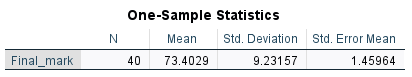
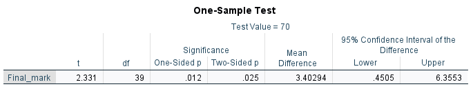
When analysing the results of the test, you should observe the descriptive statistics first in order to get an idea of what is happening in the sample. For example, the sample mean here is \(73.4029\) (displayed in the first table) as compared to \(70\) (our test value), giving a difference of \(3.4029\) (this is the mean difference in the second table). To test whether or not this difference is statistically significant requires the \(p\) value (which is listed as ‘Sig. (2-tailed)’ in the second table, as we have conducted a two-tailed hypothesis test) and the confidence interval for the difference. In terms of the \(p\) value, if we are assessing statistical significance at the \(.05\) level of significance then:
- If \(p \leqslant .05\) we reject \(\textrm{H}_\textrm{0}\) and conclude that the sample has come from a population with a mean significantly different to the test value.
- If \(p > .05\) we do not reject \(\textrm{H}_\textrm{0}\) and conclude that the sample has come from a population with a mean that is not significantly different to the test value.
In this case, our \(p\) value of \(.012\) indicates that the difference is statistically significant.
This is confirmed by the confidence interval of (\(.4505\), \(6.3553\)) for the difference between the population mean and \(70\) (our test value). Because this confidence interval does not contain zero, it again shows that the difference is statistically significant. In fact, we are \(95\%\) confident that the true population mean is between \(.4505\) and \(6.3553\) points higher than our test value.
Note that while the test statistic (\(t\)) and degrees of freedom (\(df\)) should both generally be reported as part of your results, you do not need to interpret these when assessing the significance of the difference.
If you would like to practise interpreting the results of a one sample \(t\) test for statistical significance, have a go at one or both of the following activities.
Activity 1
Activity 2
To evaluate practical significance in situations where a one sample \(t\) test is appropriate, Cohen’s \(d\) is often used to measure the effect size. This determines how many standard deviations the sample mean is from the test value, and should also be able to be obtained using statistical software. For example, the Cohen’s \(d\) for our final mark data is included in the following output:
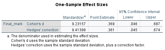
This tells us that our sample mean is \(0.369\) standard deviations from the test value, and indicates a small to medium effect (generally a Cohen’s \(d\) of magnitude \(0.2\) is considered small, \(0.5\) medium and \(0.8\) or above large).
Paired samples \(t\) test
A paired samples \(t\) test is used to test whether there is a significant difference between means for continuous variables for two related groups. For example, you would use it if you had a sample of individuals who had their heart rate recorded twice, before and after exercise, and you wanted to see if there was a significant difference between the two means. In this case the hypotheses (for a two-tailed hypothesis test) would be:
\(\textrm{H}_\textrm{0}\): There is no significant difference in heart rate before and after exercise
(\(\mu_{\textrm{HR before}} = \mu_{\textrm{HR after}}\), or \(\mu_{\textrm{HR before}} - \mu_{\textrm{HR after}} = 0\))
\(\textrm{H}_\textrm{A}\): There is a significant difference in heart rate before and after exercise
(\(\mu_{\textrm{HR before}} \neq \mu_{\textrm{HR after}}\), or \(\mu_{\textrm{HR before}} - \mu_{\textrm{HR after}} \neq 0\))
Before conducting a paired samples \(t\) test you need to check that the following assumptions are valid:
Assumption 1: The sample is a random sample that is representative of the population.
Assumption 2: The observations are independent, meaning that measurements for one subject have no bearing on any other subject’s measurements.
Assumption 3: Both variables as well as the difference variable (i.e. the differences between each data pair) are normally distributed, or the sample size is large enough that the sampling distribution of the mean approximates a normal distribution.
If the normality assumption is violated, or if you have ordinal variables rather than continuous ones (such as blood pressures recorded as low, normal or high), the Wilcoxon signed rank test should be used instead.
Assuming the assumptions for the paired samples \(t\) test are met though, and the test is conducted using statistical software (e.g. SPSS as in this example), the results should include the following statistics:
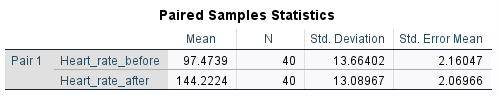
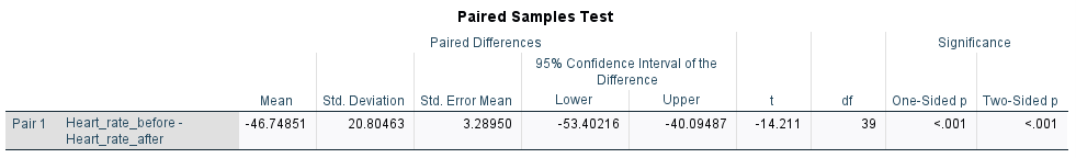
When analysing the results of the test, you should observe the descriptive statistics first in order to get an idea of what is happening in the sample. For example, the difference between the before and after sample means is \(46.74851\) (this value can be calculated from the means in the first table, and is also displayed in the second table; the fact that it is negative simply indicates that the heart rate after is greater than the heart rate before). To test whether or not this difference is statistically significant requires the \(p\) value (which is listed as ‘Sig. (2-tailed)’ in the second table, as we have conducted a two-tailed hypothesis test) and the confidence interval for the difference. In terms of the \(p\) value, if we are assessing statistical significance at the \(.05\) level of significance then:
- If \(p \leqslant .05\) we reject \(\textrm{H}_\textrm{0}\) and conclude that the means of the two related groups are significantly different.
- If \(p > .05\) we do not reject \(\textrm{H}_\textrm{0}\) and conclude that the means of the two related groups are not significantly different.
In this case, our \(p\) value of \(< .001\) indicates that the difference between the means is statistically significant.
This is confirmed by the confidence interval of (\(-53.40216\), \(-40.09487\)) for the difference between the means. Because this confidence interval does not contain zero it again means the difference is statistically significant, and in fact, we are \(95\%\) confident that the population mean heart rate after exercise is between \(40.09487\) and \(53.40216\) bpm higher than the population mean heart rate before exercise.
Note that while the test statistic (\(t\)) and degrees of freedom (\(df\)) should both generally be reported as part of your results, you do not need to interpret these when assessing the significance of the difference.
If you would like to practise interpreting the results of a paired samples \(t\) test for statistical significance, have a go at one or both of the following activities.
Activity 1
Activity 2
To evaluate practical significance in situations where a paired samples \(t\) test is appropriate, Cohen’s \(d\) can again be used to measure the effect size. This time it measures how many standard deviations the two means are separated by, and should also be able to be obtained using statistical software. For example, the Cohen’s \(d\) for our heart rate data is included in the following output:
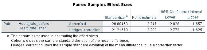
This tells us that our two sample means are separated by \(2.247\) standard deviations, and indicates a very large effect (generally a Cohen’s \(d\) of magnitude \(0.2\) is considered small, \(0.5\) medium and \(0.8\) or above large).
Independent samples \(t\) test
An independent samples \(t\) test is used to test whether there is a significant difference in means for a continuous variable for two independent groups. For example, you would use it if you collected data on hours spent watching TV each week and you wanted to see if there was a significant difference in the mean hours for males and females. In this case the hypotheses would be:
\(\textrm{H}_\textrm{0}\): There is no significant difference in TV hours per week for males and females
(\(\mu_{\textrm{males}} = \mu_{\textrm{females}}\), or \(\mu_{\textrm{males}} - \mu_{\textrm{females}} = 0\))
\(\textrm{H}_\textrm{A}\): There is a significant difference in TV hours per week for males and females
(\(\mu_{\textrm{males}} \neq \mu_{\textrm{females}}\), or \(\mu_{\textrm{males}} - \mu_{\textrm{females}} \neq 0\))
Before conducting an independent samples \(t\) test you need to check that the following assumptions are valid:
Assumption 1: The sample is a random sample that is representative of the population.
Assumption 2: The observations are independent, meaning that measurements for one subject have no bearing on any other subject’s measurements.
Assumption 3: The variable is normally distributed for both groups, or the sample size is large enough that the sampling distribution of the mean approximates a normal distribution.
If the normality assumption is violated, or if you have an ordinal variable rather than a continuous one (such as hours recorded in ranges), the Mann-Whitney U test should be used instead.
Assuming the assumptions for the independent samples \(t\) test are met though, and the test is conducted using statistical software (e.g. SPSS as in this example), the results should include the following statistics:
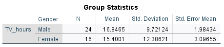
When analysing the results of the test, you should observe the descriptive statistics first in order to get an idea of what is happening in the sample. For example, the difference between the sample means for males and females is \(1.44641\) (this value can be calculated from the means in the first table, and is also displayed in the second table).
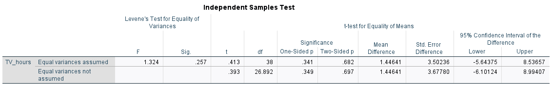
Next, note that there are actually five \(p\) values (and two confidence intervals) in the second table. Two are applicable when the variances of the two groups are approximately equal (those in the ‘One-sided p’ and ‘Two-Sided p’ columns in the top row of the table; we will interpret the ‘Two-Sided p’ value as we have conducted a two-tailed hypothesis test), two are applicable when the variances of the two groups are not approximately equal (those in the ‘One-sided p’ and ‘Two-Sided p’ columns in the bottom row of the table; we will interpret the ‘Two-Sided p’ value as we have conducted a two-tailed hypothesis test), and the remaining one (the first one in the table, in the ‘Sig.’ column) is used to determine which situation we have.
We need to interpret the latter first, which is the \(p\) value for Levene’s Test for Equality of Variances. The null hypothesis for this test is that the variances are equal, so if \(p \leqslant .05\) it is evidence to reject this null hypothesis and assume unequal variances, while if \(p > .05\) there is not enough evidence to reject the null hypothesis and equal variances can be assumed. Depending on which is which, determines which of the other \(p\) values (and confidence intervals) you should interpret. In this case, the \(p\) value of \(.257\) indicates we can assume equal variances, and that we should interpret the (two-sided) \(p\) value in the top row of the remainder of the table. Again, the interpretation of this \(p\) value is that:
- If \(p \leqslant .05\) we reject \(\textrm{H}_\textrm{0}\) and conclude that the means of the two groups are significantly different.
- If \(p > .05\) we do not reject \(\textrm{H}_\textrm{0}\) and conclude that the means of the two groups are not significantly different.
In this case, our \(p\) value of \(.682\) indicates that the difference between the means is not statistically significant.
This is confirmed by the confidence interval of (\(-5.64375\), \(8.53657\)) for the difference between the means. Because this confidence interval contains zero it again means the difference is not statistically significant, and in fact, we are \(95\%\) confident that the difference in mean hours spent watching TV each week for males and females is between \(-5.64375\) and \(8.53657\) hours.
Note that while the test statistic (\(t\)) and degrees of freedom (\(df\)) should both generally be reported as part of your results, you do not need to interpret these when assessing the significance of the difference.
If you would like to practise interpreting the results of an independent samples \(t\) test for statistical significance, have a go at one or both of the following activities.
Activity 1
Activity 2
To evaluate practical significance in situations where an independent samples \(t\) test is appropriate, Cohen’s \(d\) can again be used to measure the effect size. This time it measures how many standard deviations the two means are separated by, and should also be able to be obtained using statistical software. For example, the Cohen’s \(d\) for our heart rate data is included in the following output:
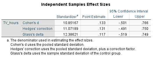
This tells us that our two sample means are separated by \(0.133\) standard deviations, and indicates a very small effect (generally a Cohen’s \(d\) of magnitude \(0.2\) is considered small, \(0.5\) medium and \(0.8\) or above large).
One-way ANOVA
One-way ANOVA is similar to the independent samples \(t\) test, but is used when three or more groups are compared. While one-way ANOVA is the only type of ANOVA covered here, note that it is just one in a family of ANOVA tests with other types including the following:
- Factorial ANOVA: used to test for differences in means between groups when there are two or more independent variables.
- One-way repeated measures ANOVA: used to test for differences in means between three or more related samples.
- ANCOVA (one-way analysis of covariance): used to test for differences between two or more independent samples after controlling for the effects of a third variable (covariate).
- MANOVA (multivariate analysis of variance): used to simultaneously test for differences between groups on multiple dependent variables.
Returning to the one-way ANOVA, consider that you have a data set containing the final marks of a sample of students studying one of three different units. You could use the one-way ANOVA to see if there is a significant difference in the mean marks for any of the units, in which case the hypotheses would be:
\(\textrm{H}_\textrm{0}\): There is no significant difference in the mean final mark for any of the three units.
(\(\mu_{\textrm{unit 1}} = \mu_{\textrm{unit 2}} = \mu_{\textrm{unit 3}}\))
\(\textrm{H}_\textrm{A}\): The mean final mark of at least one of the units is significantly different to the others.
Before conducting a one-way ANOVA you need to check that the following assumptions are valid:
Assumption 1: The sample is a random sample that is representative of the population.
Assumption 2: The observations are independent, meaning that measurements for one subject have no bearing on any other subject’s measurements.
Assumption 3: The variable is normally distributed for each of the groups, or the sample size is large enough that the sampling distribution of the mean approximates a normal distribution.
Assumption 4: The populations being compared have equal variances.
If the normality assumption is violated, or if you have an ordinal variable rather than a continuous one (such as final grade categories), the Kruskal-Wallis one-way ANOVA should be used instead. If the equal variances assumption is violated, you should use the Brown-Forsythe or Welch test instead.
Assuming the assumptions for the one-way ANOVA are met though, and the test is conducted using statistical software (e.g. SPSS as in this example), the results should include the following statistics:
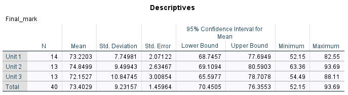
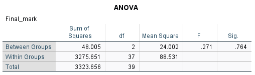
When analysing the results of the test, you should observe the descriptive statistics first in order to get an idea of what is happening in the sample. For example, the sample means are \(73.2203\) for Unit 1, \(74.8499\) for Unit 2 and \(72.1527\) for Unit 3. To test whether or not there are statistically significant differences between any of these three means requires the \(p\) value (which is listed as ‘Sig.’ in the second table), which we can interpret as follows:
- If \(p \leqslant .05\) we reject \(\textrm{H}_\textrm{0}\) and conclude that the mean of at least one of the groups is significantly different to the others.
- If \(p > .05\) we do not reject \(\textrm{H}_\textrm{0}\) and conclude that there are no significant differences between the means of any of the groups.
In this case, our \(p\) value of \(.764\) indicates that there are no significant differences in mean final grades between any of the units.
Note that while the test statistic (\(F\)) and degrees of freedom (\(df\)) should both generally be reported as part of your results, you do not need to interpret these when assessing the significance of the difference. Note also that if a one-way ANOVA is conducted and it turns out that at least one of the means is different, you will need to investigate further to determine where the difference lies using post hoc tests, for example Tukey’s HSD.
For now though, if you would like to practise interpreting the results of a one-way ANOVA for statistical significance, have a go at one or both of the following activities.
Activity 1
Activity 2
To evaluate practical significance in situations where a one-way ANOVA is appropriate, eta-squared can be used to measure the effect size. This indicates how much variability (as a percentage) in the dependent variable can be attributed to the independent variable, and should also be able to be obtained using statistical software. For example, the eta-squared for our final mark data is included in the following output:
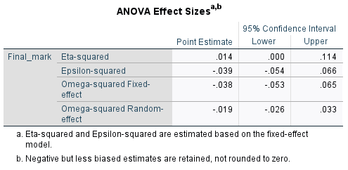
The eta-squared value of \(0.014\) tells us that \(1.4\%\) of the variability in the final marks can be attributed to the unit of study, which is a small effect (generally an eta-squared of \(0.01\) is considered small, \(0.059\) medium and \(0.138\) or above large).