Introduction to SPSS
One of the reasons you may wish to do a hypothesis test is to determine whether there is a statistically significant relationship between two or more variables, and different tests are required for this based on the type of variables.
In brief, this page covers how to do the following in SPSS:
- Conduct and interpret the output for a chi-square test of independence
- Conduct and interpret the output for a test of linear correlation
Note that the examples covered here make use of the Household energy consumption data.sav file, which contains fictitious data for 80 people based on a short ‘Household energy consumption’ questionnaire. If you want to work through the examples provided you can download the data file using the following link:
If you would like to read the sample questionnaire for which the data relates, you can do so using this link:
Before commencing the analysis, note that the default is for dialog boxes in SPSS to display any variable labels, rather than variable names. You may find this helpful, but if you would prefer to view the variable names instead then from the menu choose:
- Edit
- Options…
- Change the Variable Lists option to Display names
Testing for association
A question you may wish to ask of the wider population is: Is there a statistically significant association between having children and owning a dishwasher?
This question can be answered by following the recommended steps, as follows:
-
The appropriate hypotheses for this question are:
\(\textrm{H}_\textrm{0}\): There is no significant association between having children and owning a dishwasher
\(\textrm{H}_\textrm{A}\): There is significant association between having children and owning a dishwasher -
The appropriate test to use is a chi-square test of independence, as we are testing for association between two categorical variables (having children and owning a dishwasher).
- The assumptions for the chi-square test of independence are as follows:
- Assumption 1: The sample is a random sample that is representative of the population.
- Assumption 2: The observations are independent, meaning that measurements for one subject have no bearing on any other subject’s measurements.
- Assumption 3: The categories used for the variables are mutually exclusive.
- Assumption 4: The categories used for the variables are exhaustive.
- Assumption 5: No more than \(20\%\) of the expected frequencies are less than \(5\) (if this is violated Fisher’s exact test can be used instead).
While the first four assumptions should be met during the design and data collection phases, the fifth assumption can be checked during the analysis stage. If this assumption is violated and your variables each have only two categories, you can use the results displayed in SPSS for Fisher’s exact test instead. If your variables have more categories, you may be able to exclude or combine some of them. For instructions on combining categories by recoding, see the Transformations page of this module.
- If the first four assumptions are met, you can conduct the chi-square test of independence in SPSS by choosing the following from the SPSS menu (either from the Data Editor or Output window):
- Analyze
- Descriptive statistics
- Crosstabs…
- transfer the independent variable (‘q3’) to the Row(s) box
- transfer the dependent variable (‘q16.3’) to the Column(s) box
- select Statistics… from the right hand menu
- select Chi-square and Phi and Cramer’s V in the dialogue box
- click on Continue
- select Cells… from the right hand menu
- select Observed and Expected in the dialogue box
- click on Continue
- click on OK
The output should look like this:
-
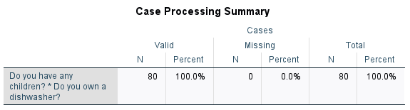
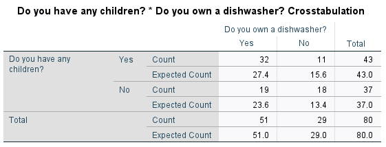
The first table simply shows that \(80\) cases have been processed. The second table shows how the actual sample data compares with what would be expected if there was no association between having children and dishwasher ownership. The fact that there is a bit of a difference between the observed and expected values provides evidence of association in the sample, with the nature of the association being that people with children are more likely to own a dishwasher.
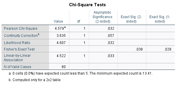
To find out whether the association is significant, we need to refer to the third table and to the ‘Asymptotic Significance (2-sided)’ value in the ‘Pearson Chi-Square’ row. Since \(p < .05\) (\(p = .032\)) we can reject the null hypothesis and conclude that there is a statistically significant association between having children and owning a dishwasher.
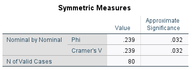
Finally, the fourth table provides the effect sizes, which can be used to test for practical significance. The ‘Phi’ of \(.239\) indicates a small to medium effect.
For more information on how to interpret these results see the Introduction to statistics module.
Testing for linear correlation
A question you may wish to ask of the wider population is: Is there a statistically significant linear correlation between summer daily energy consumption and winter daily energy consumption?
This question can be answered by following the recommended steps, as follows:
-
The appropriate hypotheses for this question are:
\(\textrm{H}_\textrm{0}\): There is no significant linear correlation between summer and winter daily energy consumption
\(\textrm{H}_\textrm{A}\): There is significant linear correlation between summer and winter daily energy consumption -
The appropriate test to use is Pearson’s correlation coefficient, as we are testing for linear correlation between two variables (summer daily energy consumption and winter daily energy consumption).
- The assumptions for Pearson’s correlation coefficient are as follows:
- Assumption 1: The sample is a random sample that is representative of the population.
- Assumption 2: The observations are independent, meaning that measurements for one subject have no bearing on any other subject’s measurements.
- Assumption 3: The variables are both continuous.
- Assumption 4: Both variables are normally distributed, or the sample size is large enough to ensure normality of the sampling distribution.
- Assumption 5: There is a linear relationship between the variables, as observed in the scatter plot (this is not strictly an assumption as Pearson’s correlation coefficient is still valid without it, but if you already know the relationship is not linear further interpretation is not necessary).
- Assumption 6: There is a homoscedastic relationship between the variables (i.e. variability in one variable is similar across all values of the other variable), as observed in the scatter plot (dots should be similar distance from line of best fit all the way along).
While the first three assumptions should be met during the design and data collection phases, the fourth, fifth and sixth assumptions should be checked at this stage (for instructions on checking the normality assumption in SPSS, see the The normal distribution page of this module).
If the normality assumption is not met you can try transforming the data or using Spearman’s Rho or Kendall’s Tau-B instead. You can also use one of these tests if you have ordinal rather than continuous variables, or if there is non-linear correlation.
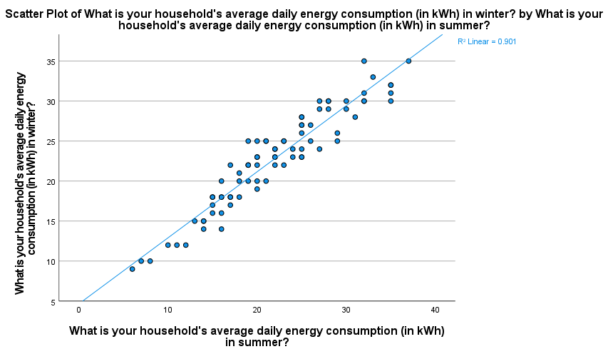
To check for linearity and homoscedasticity, you can create a scatter plot with the independent variable on the \(x\)-axis and the dependent variable on the \(y\)-axis (for this example these are interchangeable; we will put summer consumption on the \(x\)-axis). For instructions on creating a scatterplot in SPSS, see the Charts page of this module.
The scatterplot, with the line of best fit included, should look as follows. This shows that the relationship is approximately linear as the points lie close to the line of best fit. It also shows that the relationship is homoscedastic, as the points are a similar distance from the line of best fit all the way along (they don’t create a ‘funnel’ shape in either direction). Hence the fifth and sixth assumptions have been met.
- If the assumptions are met, you can assess Pearson’s correlation coefficient in SPSS by choosing the following from the SPSS menu (either from the Data Editor or Output window):
- Analyze
- Correlate
- Bivariate
- select the variables (‘q6’ and ‘q7’) and move them into the Variables box
- click on OK
The output should look like this:
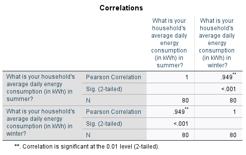
-
This table shows that Pearson’s correlation coefficient is \(.949\), indicating a strong positive linear correlation between summer and winter energy consumption (for more information on how to interpret this see the Descriptive statistics page of this module
To test whether this linear correlation is statistically significant requires the \(p\) value (listed as ‘Sig. (2-tailed)’). Since \(p < .05\) (in fact \(p < .001\)) we can reject the null hypothesis and conclude that there is a statistically significant linear correlation between summer energy consumption and winter energy consumption.
Pearson’s correlation coefficient and its square (the coefficient of variation) are also measures of effect size, which can be used to test for practical significance. The correlation coefficient of \(.949\) indicates a large effect, and the coefficient of variation of \(90.06\%\) indicates that \(90.06\%\) of variation in winter energy consumption can be explained by variation in summer energy consumption.
For more information on how to interpret these results see the Introduction to statistics module.