Introduction to SPSS
One of the reasons you may wish to do a hypothesis test is to determine whether there is a statistically significant difference between means, either for a single sample (in which case you would compare to a constant value) or for multiple independent or related samples (in which case you would compare between these different samples). Depending on the exact nature of the analysis different tests are required, and this page details the process for performing some of the most common ones using SPSS.
Conducting a one sample \(t\) test
A question you may wish to ask of the wider population is: Does this sample come from a population where the mean summer daily energy consumption is \(19\)kWh?
This question can be answered by following the recommended steps, as follows:
-
The appropriate hypotheses for this question are:
\(\textrm{H}_\textrm{0}\): The sample comes from a population with a mean summer daily energy consumption of \(19\)kWh
\(\textrm{H}_\textrm{A}\): The sample does not come from a population with a mean summer daily energy consumption of \(19\)kWh -
The appropriate test to use is the one sample \(t\) test, as we are testing whether the sample comes from a population with a specific mean (\(19\)kWh in this case).
- The assumptions for a one sample \(t\) test are as follows:
- Assumption 1: The sample is a random sample that is representative of the population.
- Assumption 2: The observations are independent, meaning that measurements for one subject have no bearing on any other subject’s measurements.
- Assumption 3: The variable is continuous.
- Assumption 4: The variable is normally distributed, or the sample size is large enough to ensure normality of the sampling distribution.
While the first three assumptions should be met during the design and data collection phases, the fourth assumption should be checked at this stage (for instructions on doing this in SPSS, see the The normal distribution page of this module). If the normality assumption is not met you can try transforming the data or conducting the One sample Wilcoxon signed-rank test instead (you can also use this test if you have an ordinal rather than continuous variable).
- If all the assumptions are met, you can conduct the one sample \(t\) test in SPSS by choosing the following from the SPSS menu (either from the Data Editor or Output window):
- Analyze
- Compare Means
- One-Sample T Test
- move the variable (‘q6’) into the Test Variable(s) box
- enter the Test Value of 19
- click on OK
The output should look like this:
-
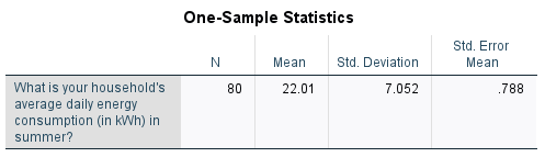
From the first table we can see that the mean summer daily energy consumption in our sample is \(22.01\)kWh, which is \(3.012\)kWh more than our hypothesised value. To test whether this is a statistically significant difference, we need to refer to the second table and to the \(p\) value and confidence interval.
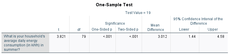
While there are actually two \(p\) values listed in the second table (the ‘One-sided \(p\)’ and ‘Two-sided \(p\)’), the standard one to use is the ‘Two-Sided \(p\)’ value as this is used to test for a difference in either direction (that is, to test whether the mean is significantly greater than or less than \(19\), as per our alternative hypothesis). Since \(p < .05\) (in fact \(p < .001\)) and since the \(95\%\) confidence interval for the difference between the population mean summer daily energy consumption and the hypothesised value does not include zero (\(95\% \textrm{CI}\) [\(1.44\)kWh, \(4.58\)kWh]), we can reject the null hypothesis and conclude that the sample actually comes from a population with mean summer daily energy consumption significantly more than \(19\)kWh.
Finally, the third table provides the effect sizes, which can be used to test for practical significance. The ‘Point Estimate’ for ‘Cohen’s \(d\)’ of \(0.427\) indicates a medium effect.
For more information on how to interpret these results see the Introduction to statistics module.
Conducting a paired samples \(t\) test
A question you may wish to ask of the wider population is: Is there a statistically significant difference between mean summer daily energy consumption and mean winter daily energy consumption?
This question can be answered by following the recommended steps, as follows:
-
The appropriate hypotheses for this question are:
\(\textrm{H}_\textrm{0}\): There is no significant difference between mean summer and winter daily energy consumption
\(\textrm{H}_\textrm{A}\): There is a significant difference between mean summer and winter daily energy consumption -
The appropriate test to use is the paired samples \(t\) test, as we are comparing the means of two related groups (summer and winter consumption for the sample people).
- The assumptions for a paired samples \(t\) test are as follows:
- Assumption 1: The sample is a random sample that is representative of the population.
- Assumption 2: The observations are independent, meaning that measurements for one subject have no bearing on any other subject’s measurements.
- Assumption 3: The variables are both continuous.
- Assumption 4: Both variables as well as the difference variable (the differences between each data pair) are normally distributed, or the sample size is large enough to ensure normality of the sampling distributions.
While the first three assumptions should be met during the design and data collection phases, the fourth assumption should be checked at this stage (for instructions on doing this in SPSS, see the The normal distribution and Transformations pages of this module). If the normality assumption is not met you can try transforming the data or conducting the Wilcoxon signed rank test instead. You can also use this test if you have ordinal rather than continuous variables.
- If all the assumptions are met, you can conduct the paired samples \(t\) test in SPSS by choosing the following from the SPSS menu (either from the Data Editor or Output window):
- Analyze
- Compare Means
- Paired-Samples T Test
- move the variables (‘q6’ and ‘q7’) into the Paired Variables box as Pair 1
- click on OK
The output should look like this:
-
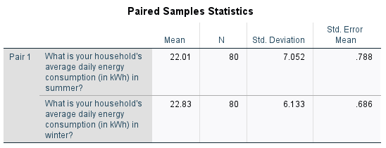
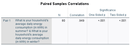
From the first table we can see that the mean summer daily energy consumption in our sample is \(22.01\)kWh, while the mean winter daily energy consumption is \(22.83\)kWh; a difference of \(0.812\)kWh. To test whether this is a statistically significant difference, we need to refer to the third table and to the \(p\) value and confidence interval. (Note that the second table provides information about the correlation between the variables, and does not need to be interpreted here.)
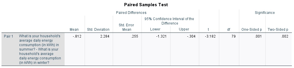
While there are actually two \(p\) values listed in the third table (the ‘One-sided \(p\)’ and ‘Two-sided \(p\)’), the standard one to use is the ‘Two-Sided \(p\)’ value as this is used to test for a difference in either direction (that is, to test whether one mean is significantly greater than or less than the other, as per our alternative hypothesis). Since \(p < .05\) (in fact \(p= .002\)) and since the \(95\%\) confidence interval for the difference between the population mean summer and winter daily energy consumptions does not include zero (\(95\% \textrm{CI}\) [\(-1.321\)kWh, \(-0.304\)kWh]), we can reject the null hypothesis and conclude that the mean summer daily energy consumption is significantly less than the mean winter daily energy consumption.
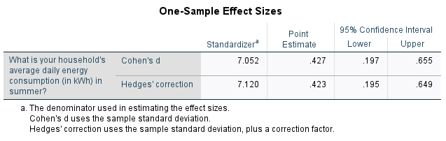
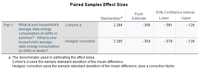
Finally, the third table provides the effect sizes, which can be used to test for practical significance. The ‘Point Estimate’ for ‘Cohen’s \(d\)’ of \(-0.356\) indicates a small to medium effect.
For more information on how to interpret these results see the Introduction to statistics module.
Conducting an independent samples \(t\) test
A question you may wish to ask of the wider population is: Is there a statistically significant difference in mean summer daily energy consumption for those with and without children?
This question can be answered by following the recommended steps, as follows:
-
The appropriate hypotheses for this question are:
\(\textrm{H}_\textrm{0}\): There is no significant difference in mean summer daily energy consumption for those with and without children
\(\textrm{H}_\textrm{A}\): There is a significant difference in mean summer daily energy consumption for those with and without children -
The appropriate test to use an independent samples \(t\) test, as we are comparing the means of two unrelated groups (summer consumption of those with and without children).
- The assumptions for an independent samples \(t\) test are as follows:
- Assumption 1: The sample is a random sample that is representative of the population.
- Assumption 2: The observations are independent, meaning that measurements for one subject have no bearing on any other subject’s measurements.
- Assumption 3: The dependent variable is continuous.
- Assumption 4: The variable is normally distributed for both groups, or the sample size is large enough to ensure normality of the sampling distribution.
While the first three assumptions should be met during the design and data collection phases, the fourth assumption should be checked at this stage (for instructions on doing this in SPSS, see the The normal distribution page of this module). If the normality assumption is not met you can try transforming the data or conducting the Mann-Whitney U test instead. You can also use this test if you have an ordinal rather than continuous dependent variable.
- If all the assumptions are met, you can conduct the independent samples \(t\) test in SPSS by choosing the following from the SPSS menu (either from the Data Editor or Output window):
- Analyze
- Compare Means
- Independent-Samples T Test
- move the continuous variable (‘q6’) into the Test Variable(s) box
- move the categorical variable (‘q3’) into the Grouping Variable box
- click on Define Groups…
- keep Group 1 as category 1 and Group 2 as category 2 and select Continue
- click on OK
The output should look like this:
-
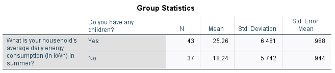
From the first table we can see that the mean summer daily energy consumption in our sample for those with children is \(25.26\)kWh, while for those without children it is \(18.24\)kWh; a difference of \(7.013\)kWh. To test whether this is a statistically significant difference, we need to refer to the second table and to the \(p\) value and confidence interval.
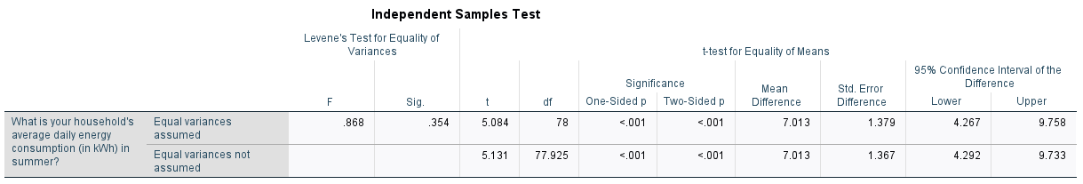
The second table actually contains five \(p\) values, of which we need to assess two. The first is for Levene’s Test for Equality of Variances (listed as ‘Sig.’), and since this \(p > .05\) (in fact \(p = .354\)), we can assume equal variances. This means we should interpret the top row of the remainder of the table. While there are actually two \(p\) values listed in the remainder of the top row (the ‘One-sided \(p\)’ and ‘Two-sided \(p\)’), the standard one to use is the ‘Two-Sided \(p\)’ value as this is used to test for a difference in either direction (that is, to test whether one mean is significantly greater than or less than the other, as per our alternative hypothesis). Since \(p < .05\) (in fact \(p < .001\)) and since the \(95\%\) confidence interval for the difference between the population mean summer daily energy consumptions of those with and without children does not include zero (\(95\% \textrm{CI}\) [\(4.267\)kWh, \(9.758\)kWh]), we can reject the null hypothesis and conclude that the mean summer daily energy consumption is significantly more for those with children compared to those without.
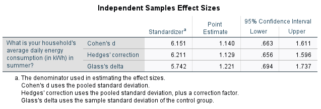
Finally, the third table provides the effect sizes, which can be used to test for practical significance. The ‘Point Estimate’ for ‘Cohen’s \(d\)’ of \(1.14\) indicates a large effect.
For more information on how to interpret these results see the Introduction to statistics module.
Conducting a one-way ANOVA
A question you may wish to ask of the wider population is: Is there a statistically significant difference in mean summer daily energy consumption for any of the different marital statuses?
This question can be answered by following the recommended steps, as follows:
-
The appropriate hypotheses for this question are:
\(\textrm{H}_\textrm{0}\): There is no significant difference in mean summer daily energy consumption for any of the different marital statuses
\(\textrm{H}_\textrm{A}\): The mean summer daily energy consumption of at least one of the marital status groups is significantly different from the others -
The appropriate test to use a one-way ANOVA, as we are comparing the means of three unrelated groups (summer consumption of those with a marital status of single, married and other).
- The assumptions for a one-way ANOVA are as follows:
- Assumption 1: The sample is a random sample that is representative of the population.
- Assumption 2: The observations are independent, meaning that measurements for one subject have no bearing on any other subject’s measurements.
- Assumption 3: The dependent variable is continuous.
- Assumption 4: The variable is normally distributed for each of the groups, or the sample size is large enough to ensure normality of the sampling distribution.
- Assumption 5: The populations being compared have equal variances.
While the first three assumptions should be met during the design and data collection phases, the fourth and fifth assumptions should be checked at this stage (for instructions on checking the normality assumption in SPSS, see the The normal distribution page of this module). Instructions on checking the equal variances assumption are included in the analysis stage.
If the normality assumption is not met you can try transforming the data or conducting the Kruskall-Wallis one-way ANOVA instead. You can also use this test if you have an ordinal rather than continuous dependent variable. If the equal variances assumption is violated you will need to use a Welch or Brown-Forsythe statistic instead.
- If the first four assumptions are met, you can conduct the one-way ANOVA in SPSS by choosing the following from the SPSS menu (either from the Data Editor or Output window):
- Analyze
- Compare Means
- One-Way ANOVA
- move the continuous variable (‘q6’) into the Dependent List box
- move the categorical variable (‘q4’) into the Factor box
- select Options… from the right hand menu
- select Descriptive and Homogeneity of variance test in the dialogue box
- click on Continue
- click on OK
The output should look like this:
-
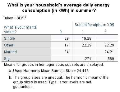
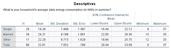
From the first table we can see that the mean summer daily energy consumption in our sample for those who are single is \(19.28\)kWh, for those who are married it is \(24.21\)kWh and for those who classified their marital status as ‘Other’ it is \(22.29\)kWh. To test whether there are any statistically significant differences between these values, we need to refer to the third table and to the \(p\) value.
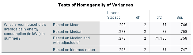
Before this though, we need to use the second table to evaluate the fifth assumption using Levene’s test of homogeneity of variance. The \(p\) value to evaluate is the one in the ‘Based on Mean’ row, which is listed as ‘Sig.’. Since this \(p > .05\) (in fact \(p = .746\)), we can assume equal variances and therefore the fifth assumption for the test is met. If the fifth assumption is not met, you can go back through the menu and keep the previous selections, but this time also select either the Brown-Forsythe test or the Welch test in the Options dialogue box.
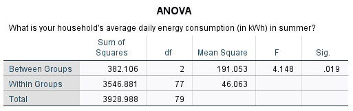
The third table contains the \(p\) value to evaluate for the one-way ANOVA, and since \(p < .05\) (in fact \(p = .019\)) we can reject the null hypothesis and conclude that the mean summer daily energy consumption is significantly different for at least one of the marital status groups.
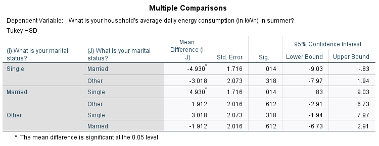
To find out where the significant difference(s) lie you can conduct a post hoc test. While there are many different options to choose from, a common test to try is Tukey’s HSD test (alternatively, if the homogeneity of variance assumption is violated you can use the Games Howell test). To do this, go back through and keep the previous selections but also do the following:
* select Post Hoc… from the right hand menu * select Tukey in the dialogue box * click on Continue * click on OKThe output should be the same as previously, but with the addition of the tables below. Both of these tables indicate that the only significant difference in mean summer daily energy consumption is between the single and married groups. This is shown by the fact that the \(p < .05\) (in fact \(p = .014\)) for this pair in the first table, and by the fact that mean values for the single and married groups do not appear in the same column of the second table.