
Introduction-to-algebra-printable-guide-UniSkills.pdf
Introduction to algebra
Table of Contents
Introduction
Welcome to the Introduction to algebra module. This module provides an overview of some key concepts in algebra, including how to rearrange and solve simple linear and quadratic equations, how to work with exponents and logarithms, and how to identify and define functions. You may wish to work your way through the entirety of the module in the order provided, or you may wish to jump to certain pages or sections of the module.
Your feedback on this module is very welcome and can be provided at any time on the feedback page, or alternatively for any questions about the module please contact Library-UniSkills@curtin.edu.au
What you will learn
- Definitions of some important algebraic terms.
- How to simplify, expand brackets, and factorise algebraic expressions.
- Techniques for rearranging and solving linear equations.
- Techniques for rearranging and solving quadratic equations.
- How to evaluate and use exponents, and how to apply exponent laws to rearrange and simplify them.
- How to convert between exponents and logarithms, how to evaluate and use logarithms, and how to apply logarithm laws to rearrange and simplify them.
- How to determine whether a relationship between input values and output values is a function, how functions are named, and the different types of functions. Key terms & techniques
In order to solve algebraic equations to find unknown values, which is a central focus of algebra, you first need to have an understanding of the key algebraic terms and techniques detailed in this page.
In brief, these are as follows:
- Definitions of some important algebraic terms
- How to simplify algebraic expressions
- How to expand brackets in algebraic expressions
- How to factorise algebraic expressions
</div>
Definitions of important terms
When a problem is written in the language of algebra we call it either an algebraic expression (when there is no equals sign), or an algebraic equation (when there is an equals sign). Both algebraic expressions and algebraic equations involve the use of constants and variables:
Constants are numbers with a fixed or constant value (for example \(1, 5, 2108, 37.5, -103,\) etc.).
</div>
Variables are small letters of the alphabet, or indeed any symbols, used to represent some unknown number in an expression or equation (for example \(x, y, a, \theta,\) etc.). The value of this number can vary (as the word variable suggests) according to the context.
</div>
In the algebraic expression \(a + 5,\) for example, \(5\) is a constant while \(a\) is a variable. This means that different numbers can be substituted for \(a\) and the value of the expression will change accordingly. For example, if \(a = 1\) then \(a + 5\) becomes \(1 + 5,\) which we know to be equal to \(6\).
Another thing to be aware of is that every ‘part’ of an algebraic expression or equation separated from other ‘parts’ by addition, subtraction or division (be it a constant, a variable or variables, or a combination of constants and variables), is referred to as a term. For example, the following algebraic expression contains \(5\) different terms, each separated by addition (note that we simply write \(x\) and \(y\) rather than \(1x\) and \(1y\), although they represent the same thing):
\[2x + y + 3y + 5x + x\]Furthermore, as this expression contains more than one variable, we say that it consists of like and unlike terms:
Like terms are terms which have the same variable. For example \(2x,\) \(5x\) and \(x\) are all like terms in the above expression. Similarly, \(y\) and \(3y\) are like terms.
Note that \(x\) and \(x^2\) are not like terms as one of the terms has an \(x\) only while the other has an \(x\) raised to the power of \(2.\) Similarly, \(x\) and \(xy\) are not like terms as one has an \(x\) only while the other has an \(x\) and a \(y.\)
</div>
Unlike terms are terms which have different variables. For example \(2x\) and \(y\) are unlike terms in the above expression. Similarly, as described above, \(x\) and \(x^2\) are unlike terms, and so too are \(x\) and \(xy\).
</div>
It is important to understand that only like terms can be added and subtracted. You wouldn’t say that \(2\) apples plus \(5\) oranges equals \(7\) apples (or \(7\) oranges), and similarly you can’t add \(2x\) and \(5y\) together.
Finally, when we combine terms together in a certain way they create polynomials:
A polynomial is an expression that consists of constants and/or variables raised to positive exponents, combined using addition, subtraction, and/or multiplication. For example, \(x^2 + 2x - 3\) is a polynomial, and so is \(20\), but \(x^{-2} + 3\) is not.
</div>
Simplifying algebraic expressions
As with most things, it is best to write an algebraic expression or equation in the simplest way possible - no need to make it any more confusing than necessary! There are a couple of key things you can do to simplify algebraic expressions and equations, and these are detailed in this section.
Note that the examples refer to algebraic expressions as it is easiest to learn the techniques with these first, but do keep in mind that the end goal is usually to apply the techniques to solve algebraic equations - as demonstrated in later pages of this module.
Adding or subtracting like terms
You can simplify an algebraic expression by adding or subtracting like terms as follows:
-
Rewrite the expression so that all like terms are next to each other. When you do this, remember to shift the \(+\) or \(–\) sign that is in front of the term with it.
-
Simplify by adding or subtracting like terms.
Example: Simplify the algebraic expression \(2a\,–\,3b\,–\,a\,+\,4ab\,–\,2b\)
Solution: Following the steps above, we have:
-
Rewriting the expression so that all like terms are next to each other gives \(2a\,–\,a\,–\,3b\,–\,2b\,+\,4ab\) (or you can write it in other ways, as long as all the \(a\) terms are together and all the \(b\) terms are together; the \(ab\) term doesn’t have any like terms)
-
Adding and subtracting the like terms in the rearranged algebraic expression \(2a\,–\,a\,–\,3b\,–\,2b\,+\,4ab\) gives \(2a\,–\,a = a\) and \(-3b\,–\,2b = -5b\), so our simplified expression is \(a\,-\,5b\,+\,4ab\)
</div>
Multiplying or dividing terms
Note that there are a few different types of notation for indicating that two (or more) terms need to be multiplied together. For example, if \(x\) and \(y\) are required to be multiplied then this might be specified as \(x \times y\), as \(x.y\), as \((x)(y)\) or as \(x(y)\).
Regardless of how the multiplication is indicated, you can simplify an algebraic expression by multiplying or dividing terms as follows:
-
Rewrite the expression (or each part of the expression, for division) as a product of its factors.
-
If necessary, rewrite the expression (or each part of the expression, for division) so that all the like terms are next to each other.
-
Multiply/divide the constants and multiply/divide the variables, as appropriate. When you do this, don’t forget that when a negative is multiplied (or divided) by a negative, the result is positive (e.g. \(-2 \times -2 = 4\)).
Example 1: Simplify the algebraic expression \(4ab \times 3acd\)
Solution: Following the steps above, we have:
-
Rewriting the expression as a product of its factors gives \(4 \times a \times b \times 3 \times a \times c \times d\)
-
Rewriting the expression so that the like terms are next to each other gives \(4 \times 3 \times a \times a \times b \times c \times d\)
-
Since \(4 \times 3 = 12\) and \(a \times a = a^2\), it follows that the simplified expression is \(12a^2bcd\)
Note that \(a^2\) is an example of an exponent (otherwise known as an indice or power). If you are unsure of how to work with exponents, it is recommended that you visit the Exponents page of this module before proceeding with further examples on this page.
</div>
Example 2: Simplify the algebraic expression \(\frac{20x^3y}{4x^2y^2}\)
Solution: Following the steps above, we have:
-
Rewriting each part of the expression as a product of its factors gives \(\frac{20 \times x \times x \times x \times y}{4 \times x \times x \times y \times y}\)
-
The like terms are already next to each other for both parts of this expression, so rewriting is not required
-
Since \(\frac{20}{4} = 5\) and \(\frac{x \times x \times x}{x \times x} = x\) and \(\frac{y}{y \times y} = \frac{1}{y}\), it follows that the simplified expression is \(\frac{5x}{y}\)
Note that the above division above has been performed by simplifying fractions, which works in the same way for variables as it does for constants. If you would like a refresher on how simplifying fractions works, please visit the Fractions section of the Numeracy fundamentals module.
</div>
Once you have worked through the examples above, have a go at simplifying some or all of the following algebraic expressions (again, please visit the Exponents page of this module first if required):
1. \(c + 5c - 2c\)
ANSWER: This expression contains all like terms, which can be added and subtracted to give \(4c\)
2. \(3d – 5c + 4 – d – 9 + 3c\)
ANSWER: Rearranging this expression gives \(3d - d - 5c + 3c + 4 - 9\), which can then be simplified to \(2d - 2c -5\)
3. \((13a)(2b)\)
ANSWER: Rewriting this expression gives \(13 \times a \times 2 \times b\), which then gives \(13 \times 2 \times a \times b\) and therefore simplifies to \(26ab\)
4. \(\frac{10a^2b}{5ac}\)
ANSWER: Rewriting this expression gives \(\frac{10 \times a \times a \times b}{5 \times a \times c}\), and since \(\frac{10}{5} = 2\) and \(\frac{a \times a}{a} = a\), it follows that it simplifies to \(\frac{2ab}{c}\)
5. \(3a + b – a – 3b\)
ANSWER: Rearranging this expression gives \(3a - a + b - 3b\), which can then be simplified to \(2a - 2b\)
6. \(2f + 3h – g + 5h + g\)
ANSWER: Rearranging this expression gives \(2f + 3h + 5h - g + g\), which can then be simplified to \(2f + 8h\)
7. \(20c – 4d + 5c + 10 – 15d\)
ANSWER: Rearranging this expression gives \(20c + 5c - 4d - 15d + 10\), which can then be simplified to \(25c - 19d + 10\)
8. \(-5f + 6 + 102g + 10f + 3\)
ANSWER: Rearranging this expression gives \(-5f + 10f + 102g + 6 + 3\), which can then be simplified to \(5f + 102g + 9\)
9. \(4c \times ab \times 9\)
ANSWER: Rewriting this expression gives \(4 \times c \times a \times b \times 9\), which then gives \(4 \times 9 \times c \times a \times b\) and therefore simplifies to \(36abc\) (while the variables can be listed in any order, the usual convention is to list them alphabetically)
10. \(2a \times a \times 5a^2\)
ANSWER: Rewriting this expression gives \(2 \times a \times a \times 5 \times a \times a\), which then gives \(2 \times 5 \times a \times a \times a \times a\) and therefore simplifies to \(10a^4\)
11. \(\frac{12ac}{ab}\)
ANSWER: Rewriting this expression gives \(\frac{12 \times a \times c}{a \times b}\), and since \(\frac{a}{a} = 1\), it follows that it simplifies to \(\frac{12c}{b}\)
12. \(\frac{20d^2ef}{5de}\)
ANSWER: Rewriting this expression gives \(\frac{20 \times d \times d \times e \times f}{5 \times d \times e}\), and since \(\frac{20}{5} = 4\) and \(\frac{d \times d}{d} = d\) and \(\frac{e}{e} = 1\), it follows that it simplifies to \(4df\)
Expanding brackets
Often an algebraic expression or equation contains brackets. When this is the case for an equation, sometimes it can be helpful to expand them in order to solve it. This section details how to do this for both one and two sets of brackets (note again that the examples refer to algebraic expressions rather than equations for simplicity; applying the techniques as part of solving algebraic equations will be demonstrated in later pages of this module).
Expanding one set of brackets
An algebraic expression consisting of a term outside one set of brackets can be expanded as follows:
-
Write out each of the multiplications you need to perform, by putting the term outside the brackets together with each term inside the brackets. If you use the multiplication notation of putting brackets around each term when you do this, then you can simply add each pair of terms together and deal with any negative signs later.
-
Perform each of the required multiplications, using the method described previously, again leaving each result in brackets in order to keep track of any negative signs. These will be dealt with next.
-
Remove the brackets from each term, replacing a positive sign with a negative sign if there is one inside the corresponding set of brackets.
Example: Expand the brackets in the algebraic expression \(-3a(2b + 4a - 9)\)
Solution: Following the steps above, we have:
-
Writing out the multiplications we need to perform, using brackets to indicate multiplication and adding each pair of terms, gives \((-3a)(2b) + (-3a)(4a) + (-3a)(-9)\)
-
Performing the multiplication above, keeping the results in brackets, gives \((-6ab) + (-12a^2) + (27a)\)
-
Removing brackets and making the required terms negative gives \(-6ab - 12a^2 + 27a\)
Note that \(a^2\) is an example of an exponent (otherwise known as an indice or power). If you are unsure of how to work with exponents, it is recommended that you visit the Exponents page of this module before proceeding with further examples on this page.
</div>
Expanding pairs of brackets
An algebraic expression consisting of two sets of brackets that are being multiplied together can be expanded as follows:
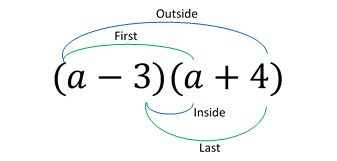
- Write out each of the multiplications you need to perform, by putting each term in the first set of brackets with each term in the second set of brackets and adding these terms together. Again, use brackets to indicate multiplication and add each pair of terms to avoid any confusion with negative signs. Note that a handy way of remembering which terms to multiply when there are two terms in each set of brackets is with the acronym FOIL, which stands for:
- First: Multiply the first terms in each bracket
- Outside: Multiply the two outside terms
- Inside: Multiply the two inside terms
-
Last: Multiply the last terms in each bracket
\(\)
-
Perform each of the required multiplications, leaving each result in brackets in order to keep track of any negative signs. These will be dealt with in the next step.
-
Remove the brackets from each term, replacing the positive sign with a negative sign if there is one inside the corresponding set of brackets.
- Simplify the expression by adding and/or subtracting like terms as required (as detailed in the above section).
Example: Expand the brackets in the algebraic expression \((a - 3)(a + 4)\)
Solution: Following the steps above, we have:
-
Writing out the multiplications we need to perform, using brackets to indicate multiplication and adding each pair of terms, gives \((a)(a) + (a)(4) + (-3)(a) + (-3)(4)\)
Again note that FOIL can help with this:
-
Performing the multiplication above, keeping the results in brackets, gives \((a^2) + (4a) + (-3a) + (-12)\)
-
Removing brackets and making the required terms negative gives \(a^2 + 4a - 3a - 12\)
-
Finally, simplifying the expression gives \(a^2 + a - 12\)
</div>
Once you have worked through the examples above, have a go at expanding brackets in the following algebraic expressions (again, please visit the Exponents page of this module first if required):
1. \(b(3 + b)\)
\(= (b)(3) + (b)(b)\)
\(= 3b + b^2\)
2. \(3xy(6x - y^2 + x^2y)\)
\(= (3xy)(6x) + (3xy)(-y^2) + (3xy)(x^2y)\)
\(= 18x^2y) + (-3xy^3) + (3x^3y^2)\)
\(= 18x^2y - 3xy^3 + 3x^3y^2\)
3. \((e + f)(g + f)\)
\(= (e)(g) + (e)(f) + (f)(g) + (f)(f)\)
\(= eg + ef + fg + f^2\)
4. \((c - 4d)(-c - 3d)\)
\(= (c)(-c) + (c)(-3d) + (-4d)(-c) + (-4d)(-3d)\)
\(= (-c^2) + (-3cd) + (4cd) + (12d^2)\)
\(= -c^2 - 3cd + 4cd + 12d^2\)
\(= -c^2 + cd + 12d^2\)
5. \(a(-a +1 – ac^2) \)
\(= (a)(-a) + (a)(1) + (a)(-ac^2)\)
\(= (-a^2) + (a) + (-a^2c^2)\)
\(= -a^2 + a - a^2c^2\)
6. \(–3d(3 – 2c + 5d)\)
\(= (-3d)(3) + (-3d)(-2c) + (-3d)(5d)\)
\(= (-9d) + (6cd) + (-15d^2)\)
\(= -9d + 6cd - 15d^2\)
7. \(–a^3(-a^2 – 3a + 4)\)
\(= (-a^3)(-a^2) + (-a^3)(-3a) + (-a^3)(4)\)
\(= (a^5) + (3a^4) + (-4a^3)\)
\(= a^5 + 3a^4 - 4a^3\)
8. \(4dg^2(2d + 3g^3)\)
\(= (4dg^2)(2d) + (4dg^2)(3g^3)\)
\(= 8d^2g^2 + 12dg^5\)
9. \((7x + 2y)(8x – 3y)\)
\(= (7x)(8x) + (7x)(-3y) + (2y)(8x) + (2y)(-3y)\)
\(= (56x^2) + (-21xy) + (16xy) + (-6y^2)\)
\(= 56x^2 - 21xy + 16xy - 6y^2\)
\(= 56x^2 - 5xy - 6y^2\)
10. \((x^2 + y)(x + y)\)
\(=(x^2)(x) + (x^2)(y) + (y)(x) + (y)(y)\)
\(= x^3 + x^2y + xy + y^2\)
11. \((x + 3y)(2x – 4)\)
\(= (x)(2x) + (x)(-4) + (3y)(2x) + (3y)(-4)\)
\(= (2x^2) + (-4x) + (6xy) + (-12y)\)
\(= 2x^2 - 4x + 6xy - 12y\)
12. \((2x + 3)(2x – 1)\)
\(= (2x)(2x) + (2x)(-1) + (3)(2x) + (3)(-1)\)
\(= (4x^2) + (-2x) + (6x) + (-3)\)
\(= 4x^2 - 2x + 6x - 3\)
\(= 4x^2 + 4x - 3\)
Factorising
Factorising is essentially the opposite of expanding brackets; instead of removing brackets, you put them into an algebraic expression or equation. Factorising is another tool that you can use to help you solve algebraic equations in certain situations (although obviously, it wouldn’t help to go back and forth expanding and factorising the same equation!).
This section details how to factorise using one set of brackets, and at a common example of factorising using two sets of brackets (note again that the examples refer to algebraic expressions rather than equations for simplicity; applying the techniques as part of solving algebraic equations will be demonstrated in later pages of this module).
Factorising with one set of brackets
You can factorise an algebraic expression using one set of brackets as follows:
-
Identify the highest common factor for all terms in the expression (where the highest common factor is the largest term that divides into each term in the expression). This may be a constant or a variable or variables, or a combination of both.
-
Put the highest common factor outside of a set of brackets.
-
Put what remains of each term in the original expression inside the brackets.
Example: Factorise the algebraic expression \(3x^2 + 21x\)
Solution: Following the steps above, we have:
-
The highest common factor is \(3x\), since \(3\) divides into each term in the expression a whole number of times and there is one \(x\) in each term.
-
Putting this outside a set of brackets gives \(3x(…..)\)
-
Since there is an \(x\) remaining in \(3x^2\) when it is divided through by \(3x\), the first term inside the brackets should be \(x\).
Since there is a \(7\) remaining in \(21x\) when it is divided through by \(3x\), the second term inside the brackets should be \(7\).
Therefore it follows that the factorised form of the expression is \(3x(x + 7)\)
Note that \(x^2\) is an example of an exponent (otherwise known as an indice or power). If you are unsure of how to work with exponents, it is recommended that you visit the Exponents page of this module before proceeding with further examples on this page.
</div>
Factorising with two sets of brackets
Sometimes two sets of brackets are required to factorise an expression. A common example of this is when factorising a quadratic, which is an algebraic expression of the form \(ax^2 + bx + c\) (where \(a\), \(b\) and \(c\) are numbers, and \(a\) does not equal 0 - as this would not be a quadratic).
For more information on quadratic equations see the Solving quadratic equations page of this module, but in the meantime know that you can factorise a quadratic equation for which \(a = 1\) as follows:
-
Write two sets of brackets, and put the variable used in the expression inside both.
-
Determine pairs of factors for the last term in the expression, taking into account whether these factors are positive or negative.
-
Determine which of these pairs of factors can be added together or subtracted from one another to give the constant associated with the middle term in the expression. Then write one of these in each of the sets of brackets, being sure to use appropriate signs.
Example: Factorise the algebraic expression \(x^2 + 7x + 12\)
Solution: Following the steps above, we have:
-
Writing out two sets of brackets with the variable inside each gives \((x\textrm{…..})(x\textrm{…..})\)
-
The pairs of factors for \(12\) are \(1\) and \(12\), \(2\) and \(6\) and \(3\) and \(4\). Note that both terms must be positive, since they need to multiply together to make positive \(12\) and add together to make positive \(7\)
-
The pair of factors that can be added together to make \(7\) is \(3\) and \(4\), so the factorised form of \(x^2 + 7x + 12\) is \((x + 3)(x + 4)\), or \((x + 4)(x + 3)\) (it doesn’t matter which way around you write it)
</div>
Once you have worked through the examples above, have a go at factorising the following algebraic expressions (again, please visit the Exponents page of this module first if required):
1. \(14a + 8ab\)
Common factor is \(2a\), so factorising gives \(2a(7 + 4b)\)
2. \(12x^3y – 3x^2y^2 + 6x^2yz\)
Common factor is \(3x^2y\), so factorising gives \(3x^2y(4x - y + 2z)\)
3. \(x^2 + x – 12\)
This is a quadratic so we need two sets of brackets, and two numbers that multiply together to make \(-12\) and add together to make \(1\) (since \(x = 1x\)). The factors of \(12\) are \(1\) & \(12\), \(2\) & \(6\) and \(3\) & \(4\), and one of each pair must be negative and one positive in order to multiply together to make \(-12\). The correct pair is \(-3\) and \(4\), since \(-3 + 4 = 1\), so the expression can be factorised as \((x - 3)(x + 4)\)
4. \( y^2 – 8y + 12\)
This is a quadratic so we need two sets of brackets, and two numbers that multiply together to make \(12\) and add together to make \(-8\). The factors of \(12\) are \(1\) & \(12\), \(2\) & \(6\) and \(3\) & \(4\), and both numbers must be negative in order to multiply together to make \(12\) and add together to make \(-8\). The correct pair is \(-2\) and \(-6\), since \(-2 - 6 = -8\), so the expression can be factorised as \((y - 2)(y - 6)\)
5. \(z^2 – 4z – 12\)
This is a quadratic so we need two sets of brackets, and two numbers that multiply together to make \(-12\) and add together to make \(-4\). The factors of \(12\) are \(1\) & \(12\), \(2\) & \(6\) and \(3\) & \(4\), and one of each pair must be negative and one positive in order to multiply together to make \(-12\). The correct pair is \(2\) and \(-6\), since \(2 - 6 = -4\), so the expression can be factorised as \((z + 2)(z - 6)\)
6. \(10c + 15c^2\)
Common factor is \(5c\), so factorising gives \(5c(2 + 3c)\)
7. \(16abc + 4ac – 12abc^2\)
Common factor is \(4ac\), so factorising gives \(4ac(4b + 1 - 3bc)\)
8. \(3mn + 6m^2 – 12mn^2\)
Common factor is \(3m\), so factorising gives \(3m(n + 2m - 4n^2)\)
9. \(-5x^2y – 10x^3 – 20x^2\)
Common factor is \(-5x^2\), so factorising gives \(-5x^2(y + 2x + 4)\)
10. \(x^2 + 5x + 6\)
This is a quadratic so we need two sets of brackets, and two numbers that multiply together to make \(6\) and add together to make \(5\). The factors of \(6\) are \(1\) & \(6\) and \(2\) & \(3\), and both numbers must be positive in order to multiply together to make \(6\) and add together to make \(5\). The correct pair is \(2\) and \(3\), since \(2 + 3 = 5\), so the expression can be factorised as \((x + 2)(x + 3)\)
11. \(y^2 - 3y – 10\)
This is a quadratic so we need two sets of brackets, and two numbers that multiply together to make \(-10\) and add together to make \(-3\). The factors of \(10\) are \(1\) & \(10\) and \(2\) & \(5\), and one of each pair must be negative and one positive in order to multiply together to make \(-10\). The correct pair is \(2\) and \(-5\), since \(2 - 5 = -3\), so the expression can be factorised as \((y + 2)(y - 5)\)
12. \(a^2 - 10a + 24\)
This is a quadratic so we need two sets of brackets, and two numbers that multiply together to make \(24\) and add together to make \(-10\). The factors of \(24\) are \(1\) & \(24\), \(2\) & \(12\), \(3\) & \(8\) and \(4\) & \(6\), and both numbers must be negative in order to multiply together to make \(24\) and add together to make \(-10\). The correct pair is \(-6\) and \(-4\), since \(-6 - 4 = -10\), so the expression can be factorised as \((a - 6)(a - 4)\)
13. \(b^2 - b – 20\)
This is a quadratic so we need two sets of brackets, and two numbers that multiply together to make \(-20\) and add together to make \(-1\). The factors of \(20\) are \(1\) & \(20\), \(2\) & \(10\) and \(4\) & \(5\), and one of each pair must be negative and one positive in order to multiply together to make \(-20\). The correct pair is \(4\) and \(-5\), since \(4 - 5 = -1\), so the expression can be factorised as \((b + 4)(b - 5)\)
14. \(c^2 + 2c + 1\)
This is a quadratic so we need two sets of brackets, and two numbers that multiply together to make \(1\) and add together to make \(2\). The only factors of \(1\) are \(1\) & \(1\), and we need both of these to be positive in order to multiply together to make \(1\) and add together to make \(2\). Hence the expression can be factorised as \((c + 1)(c + 1)\), which we would usually write as \((c + 1)^2\)
15. \(d^2 + d – 30\)
This is a quadratic so we need two sets of brackets, and two numbers that multiply together to make \(-30\) and add together to make \(1\). The factors of \(30\) are \(1\) & \(30\), \(2\) & \(15\), \(3\) & \(10\) and \(5\) & \(6\), and one of each pair must be negative and one positive in order to multiply together to make \(-30\). The correct pair is \(6\) and \(-5\), since \(6 - 5 = 1\), so the expression can be factorised as \((d + 6)(d - 5)\)
Linear equations
Once you have an understanding of some key algebraic terms and techniques you can apply them to solve linear equations, as detailed in this page.
In brief, it covers the following:
- The definition of a linear equation
- How to rearrange a linear equation
- How to solve a linear equation in one variable
- How to write a linear equation in slope-intercept form
</div>
What is a linear equation?
Recall that an algebraic equation is just like an algebraic expression, but it also contains an equals (\(=\)) sign. For example, \(5 + d\) is an algebraic expression, while \(5 + d = 10\) is an algebraic equation. A particular kind of algebraic equation is a linear equation, or first degree equation:
A linear equation is an equation that only has variables raised to the first power, for example \(a\,–\,3 = 5\) as opposed to \(a^2\,–\,3 = 5\)
</div>
A linear equation with only one variable is called a linear equation in one variable, a linear equation with two variables is called a linear equation in two variables, and so on.
When we have a linear equation in one variable, we can determine the value of that variable and hence solve the equation by rearranging it so that the variable is by itself on one side of the equals sign. For example, to solve the equation \(c + 2 = 5\) you just need to get \(c\) by itself on one side of the equals sign.
Note that you can also solve linear equations in two or more variables, but this requires you to have the same number of equations as you do variables. Doing this is referred to as solving simultaneous equations, but this is not covered here (if you are interested in learning about how to do this, one example of a page you might find helpful is https://www.mathsisfun.com/algebra/systems-linear-equations.html).
Rearranging linear equations
Rearranging a linear equation in one variable in order to solve it requires you to ‘get rid of’ constants that are around the variable, that is, constants that have been added to it or that it has been multiplied by, for example. To do this, you need to undo whatever has been done with the constant by performing an ‘opposite’ operation. For example you might:
| Remove a constant that was… | By… |
|---|---|
| Added | Subtracting it |
| Subtracted | Adding it |
| Multiplied by | Dividing by it |
| Divided by | Multiplying by it |
The important thing to remember here is that whichever operation or operations you perform on one side of the equation, you must also do on the other side! This way you keep the equation in balance.

In other words, whatever you do to one side of an equation you need to do to the other side in the same step of working. For example:
| On the left hand side (LHS) of \(=\), if you… | On the right hand side (RHS) of \(=\), you must… |
|---|---|
| Add \(2\) (\(+2\)) | Add \(2\) (\(+2\)) |
| Subtract \(5\) (\(-5\)) | Subtract \(5\) (\(-5\)) |
| Multiply by \(7\) (\(\times 7\)) | Multiply by \(7\) (\(\times 7\)) |
| Divide by \(3\) (\(\div 3\)) | Divide by \(3\) (\(\div 3\)) |
Going back to the equation \(c + 2 = 5\), and to solve it you would undo the addition of \(2\) by subtracting \(2\) from both sides of the equation, as follows (note that with such a simple equation you don’t really need to use these techniques, but they will come in really handy with more complex equations - and it’s always best to start with a simple example!):
\[\begin{aligned} && c + 2 &= 5 \\\ \therefore && c + 2 - 2 &= 5 - 2 && \textrm{ (undo addition by subtracting) } \\\ \therefore && c &= 3 && \textrm{ (simplify - equation is solved!) } \end{aligned}\]Note that the \(\therefore\) sign shown above is just shorthand for ‘therefore’.
At this point, it is worth being aware of the fact that as you become more familiar with solving equations, you will find different ways of writing out your working that make sense to you. These may be slightly different to what is shown above, and that’s fine (as long as they are correct of course). For example, you may prefer to think of the ‘plus \(2\)’ as merely switching sides and becoming ‘subtract \(2\)’, as follows:
\[\begin{aligned} && c + 2 &= 5 \\\ \therefore && c &= 5 - 2 && \textrm{ (addition of }2\textrm{ on left becomes subtraction of }2\textrm{ on right)} &\\\ \therefore && c &= 3 && \textrm{ (simplify - equation is solved!)} \end{aligned}\]Steps for solving linear equations
Often multiple operations need to be undone in order to solve a linear equation in one variable. While this can require a bit of thought for complex equations, and as noted previously there are sometimes different techniques for solving the same equation, a general starting point is to follow these steps:
-
If your equation has brackets in it, expand these first (if you need a refresher on how to do this, refer to the Key terms and techniques page of this module).
-
If your equation has like terms in it, group these together next (adding or subtracting them from one side of the equation if required) and then simplify the equation (again, refer to the Key terms and techniques page of this module if required).
- If your equation requires more than one constant to be removed from the variable, undo one operation at a time in the following order:
- Remove anything that has been added to or subtracted from the variable
- Remove anything that the variable has been multiplied or divided by
- Check that the answer you have obtained is actually correct, by substituting the value back into the original equation and evaluating it. If it’s not correct, go back and see if you can find where you went wrong and work through the steps again.
Example: Solve the linear equation \(10d - 2 = 7(d + 1)\)
Solution: Following the steps above, we have:
\[\begin{aligned} && 10d - 2 &= 7(d + 1) \\\ \therefore && 10d - 2 &= 7d + 7 && \textrm{ (expand brackets)} \\\ \therefore && 10d - 2 - 7d &= 7d + 7 - 7d && \textrm{ (remove variable from RHS of equation by subtracting)} \\\ \therefore && 3d - 2 &= 7 && \textrm{ (simplify)} \\\ \therefore && 3d - 2 + 2 &= 7 + 2 && \textrm{ (undo subtraction by adding)} \\\ \therefore && 3d &= 9 && \textrm{ (simplify)} \\\ \therefore && 3d/3 &= 9/3 && \textrm{ (undo multiplication by dividing)} \\\ \therefore && d &= 3 && \textrm{ (simplify - equation is solved!)} \end{aligned}\]Finally, substituting \(3\) back into the original equation gives \((10)(3) - 2 = 30 - 2 = 28\) on the left hand side, and \(7(3 + 1) = 7(4) = 28\) on the right hand side. So the solution is correct.
</div>
Once you have worked through the example above, have a go at solving some or all of the following linear equations:
1. Solve \(c + 3 = 9\) to find the value of \(c\)
\(\begin{aligned} && c + 3 &= 9 \\\ \therefore && c + 3 - 3 &= 9 - 3 && \textrm{ (undo addition by subtracting)} \\\ \therefore && c &= 6 && \textrm{ (simplify - equation is solved!)} \end{aligned}\)
2. Solve \(\frac{a}{3} = 2\) to find the value of \(a\)
\(\begin{aligned} && \frac{a}{3} &= 2 \\\ \therefore && 3(\frac{a}{3}) &= 3(2) && \textrm{ (undo division by multiplying)} \\\ \therefore && a &= 6 && \textrm{ (simplify - equation is solved!)} \end{aligned}\)
3. Solve \(3p + 2 = 17\) to find the value of \(p\)
\(\begin{aligned} && 3p + 2 &= 17 \\\ \therefore && 3p + 2 - 2 &= 17 - 2 && \textrm{ (undo addition by subtracting)} \\\ \therefore && 3p &= 15 && \textrm{ (simplify)} \\\ \therefore && \frac{3p}{3} &= \frac{15}{3} && \textrm{ (undo multiplication by dividing)} \\\ \therefore && p &= 5 && \textrm{ (simplify - equation is solved!)} \end{aligned}\)
4. Solve \(3y - 5 = 13\) to find the value of \(y\)
\(\begin{aligned} && 3y - 5 &= 13 \\\ \therefore && 3y - 5 + 5 &= 13 + 5 && \textrm{ (undo subtraction by adding)} \\\ \therefore && 3y &= 18 && \textrm{ (simplify)}& \\\ \therefore && \frac{3y}{3} &= \frac{18}{3} && \textrm{ (undo multiplication by dividing)} \\\ \therefore && p &= 6 && \textrm{ (simplify - equation is solved!)} \end{aligned}\)
5. Solve \(3a + 4 = a + 6\) to find the value of \(a\)
\(\begin{aligned} && 3a + 4 &= a + 6 \\\ \therefore && 3a + 4 - a &= a + 6 - a && \textrm{ (remove variable from RHS by subtracting)} \\\ \therefore && 2a + 4 &= 6 && \textrm{ (simplify)} \\\ \therefore && 2a + 4 - 4 &= 6 - 4 && \textrm{ (undo addition by subtracting)} \\\ \therefore && 2a &= 2 && \textrm{ (simplify)} \\\ \therefore && \frac{2a}{2} &= \frac{2}{2} && \textrm{ (undo multiplication by dividing)} \\\ \therefore && a &= 1 && \textrm{ (simplify - equation is solved!)} \end{aligned}\)
6. Solve \(6n = 20 + 2n\) to find the value of \(n\)
\(\begin{aligned} && 6n &= 20 + 2n \\\ \therefore && 6n - 2n &= 20 + 2n - 2n && \textrm{ (remove variable from RHS by subtracting)} \\\ \therefore && 4n &= 20 && \textrm{ (simplify)} \\\ \therefore && \frac{4n}{4} &= \frac{20}{4} && \textrm{ (undo multiplication by dividing)} \\\ \therefore && n &= 5 && \textrm{ (simplify - equation is solved!)} \end{aligned}\)
7. Solve \(5a – 5 + 10a = -5\) to find the value of \(a\)
\(\begin{aligned} && 5a - 5 + 10a &= -5 \\\ \therefore && 15a - 5 &= -5 && \textrm{ (simplify like terms)} \\\ \therefore && 15a - 5 + 5 &= -5 + 5 && \textrm{ (undo subtraction by adding)} \\\ \therefore && 15a &= 0 && \textrm{ (simplify)} \\\ \therefore && \frac{15a}{15} &= \frac{0}{15} && \textrm{ (undo multiplication by dividing)} \\\ \therefore && a &= 0 && \textrm{ (simplify - equation is solved!)} \end{aligned}\)
8. Solve \(5(d - 2) = 10\) to find the value of \(d\)
\(\begin{aligned} && 5(d - 2) &= 10 \\\ \therefore && 5d - 10 &= 10 && \textrm{ (expand brackets)} \\\ \therefore && 5d - 10 + 10 &= 10 + 10 && \textrm{ (undo subtraction by adding)} \\\ \therefore && 5d &= 20 && \textrm{ (simplify)} \\\ \therefore && \frac{5d}{5} &= \frac{20}{5} && \textrm{ (undo multiplication by dividing)} \\\ \therefore && d &= 4 && \textrm{ (simplify - equation is solved!)} \end{aligned}\)
9. Solve \(3(d - 4) = 12\) to find the value of \(d\)
\(\begin{aligned} && 3(d - 4) &= 12 \\\ \therefore && 3d - 12 &= 12 && \textrm{ (expand brackets)} \\\ \therefore && 3d - 12 + 12 &= 12 + 12 && \textrm{ (undo subtraction by adding)} \\\ \therefore && 3d &= 24 && \textrm{ (simplify)} \\\ \therefore && \frac{3d}{3} &= \frac{24}{3} && \textrm{ (undo multiplication by dividing)} \\\ \therefore && d &= 8 && \textrm{ (simplify - equation is solved!)} \end{aligned}\)
10. Solve \(\frac{2a - 1}{6} = 4\) to find the value of \(a\)
\(\begin{aligned} && \frac{2a - 1}{6} &= 4 \\\ \therefore && 2a - 1 &= 24 && \textrm{ (simplify)} \\\ \therefore && 2a - 1 + 1 &= 24 + 1 && \textrm{ (undo subtraction by adding)} \\\ \therefore && 2a &= 25 && \textrm{ (simplify)} \\\ \therefore && \frac{2a}{2} &= \frac{25}{2} && \textrm{ (undo multiplication by dividing)} \\\ \therefore && a &= 12.5 && \textrm{ (simplify - equation is solved!)} \end{aligned}\)
11. Solve \(\frac{-2t + 1}{3} + 2 = 6\) to find the value of \(t\)
\(\begin{aligned} && \frac{-2t + 1}{3} + 2 &= 6 \\\ \therefore && \frac{-2t + 1}{3} + 2 - 2 &= 6 - 2 && \textrm{ (undo addition by subtracting)} \\\ \therefore && \frac{-2t + 1}{3} &= 4 && \textrm{ (simplify)} \\\ \therefore && 3(\frac{-2t + 1}{3}) &= 3(4) && \textrm{ (undo division by multiplying)} \\\ \therefore && -2t + 1 &= 12 && \textrm{ (simplify)} \\\ \therefore && -2t + 1 - 1 &= 12 - 1 && \textrm{ (undo addition by subtracting)} \\\ \therefore && -2t &= 11 && \textrm{ (simplify)} \\\ \therefore && \frac{-2t}{-2} &= \frac{11}{-2} && \textrm{ (undo multiplication by dividing)} \\\ \therefore && t &= -5.5 && \textrm{ (simplify - equation is solved!)} \end{aligned}\)
Slope-intercept form
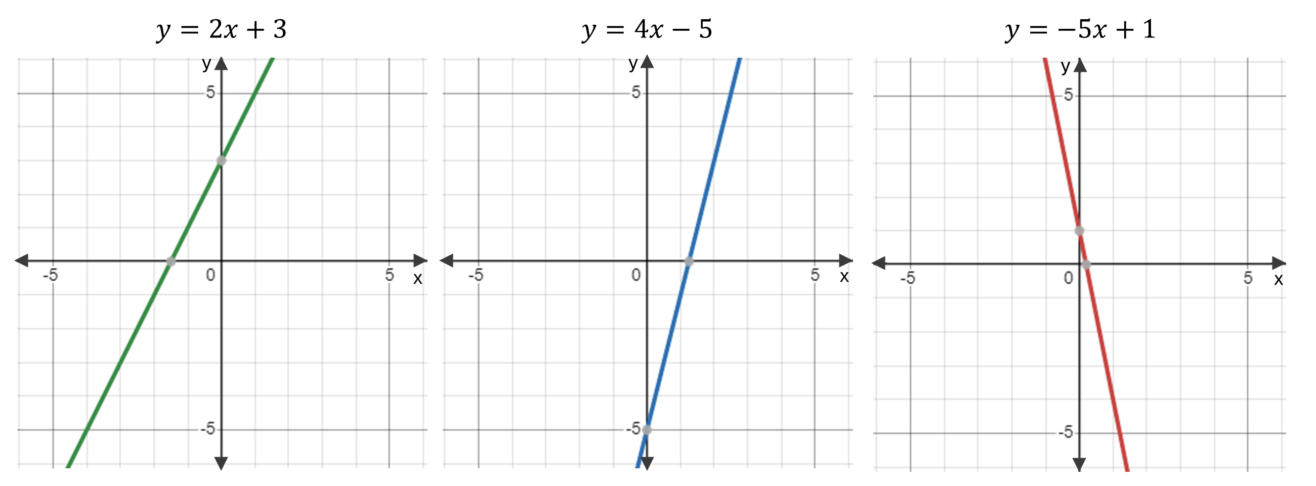
When you plot a linear equation in two variables on a graph it forms a straight line. The most common way to write this kind of equation is in a format that clearly indicates two key properties of the line, and this is called slope-intercept form. It is as follows:
\[y = mx + c\]where:
- \(m\) is the gradient or slope of the line (for more on the gradient see the Derivatives page of the Introduction to calculus module)
- \(c\) is the y-intercept (the point where the line intercepts the y-axis, or vertical axis).
For example, the following linear equations are all in slope-intercept form:
\(y = 2x + 3\)
\(y = 4x - 5\)
\(y = -5x + 1\)
The graphs of these equations are as shown (note the different gradients and y-intercepts):
If a linear equation in two variables is not in slope-intercept form, it can be rearranged into this form by following the techniques described for solving linear equations.
Example: Rearrange the linear equation \(6x + 2y = 10\) to be in slope-intercept form.
Solution: Rearranging using the steps for solving linear equations gives:
\[\begin{aligned} && 6x + 2y &= 10 \\\ \therefore && 6x + 2y - 6x &= 10 - 6x && \textrm{ (remove } 6x \textrm{ from LHS of equation by subtracting)} \\\ \therefore && 2y &= 10 - 6x && \textrm{ (simplify)} \\\ \therefore && 2y/2 &= 10/2 - 6x/2 && \textrm{ (undo multiplication by dividing)} \\\ \therefore && y &= 5 - 3x && \textrm{ (simplify)} \\\ \therefore && y &= - 3x + 5&& \textrm{ (rearrange)} \end{aligned}\]</div>
Once you have worked through the example above, have a go at some or all of these problems involving linear equations in slope-intercept form:
1. State the gradient and y-intercept of the straight line \(y = 3x - 4\)
The gradient of this line is \(3\) and the y-intercept is \(-4\)
2. State the gradient and y-intercept of the straight line \(y = -0.4x + 7\)
The gradient of this line is \(-0.4\) and the y-intercept is \(7\)
3. Rearrange the linear equation \(-12x = 6 - 3y\)
\(\begin{aligned} && -12x &= 6 - 3y \\\ \therefore && -12x + 3y &= 6 - 3y + 3y && \textrm{ (remove }-3y \textrm{ from RHS of equation by adding} \\\ \therefore && -12x + 3y &= 6 && \textrm{ (simplify)} \\\ \therefore && -12x + 3y + 12x &= 6 + 12x && \textrm{ (remove }-12x \textrm{ from LHS of equation by adding} \\\ \therefore && 3y &= 6 + 12x && \textrm{ (simplify)} \\\ \therefore && 3y/3 &= 6/3 + 12x/3 && \textrm{ (undo multiplication by dividing)} \\\ \therefore && y &= 4x + 2 && \textrm{ (simplify and rearrange)} \\\ \end{aligned}\)
4. Rearrange the linear equation \(4y + 20x + 8 = 0\)
\(\begin{aligned} && 4y + 20x + 8 &= 0 \\\ \therefore && 4y + 20x + 8 - 8 &= 0 - 8 && \textrm{ (remove } 8 \textrm{ from LHS of equation by subtracting} \\\ \therefore && 4y + 20x &= -8 && \textrm{ (simplify)} \\\ \therefore && 4y + 20x - 20x &= -8 - 20x && \textrm{ (remove } 20x \textrm{ from LHS of equation by subtracting} \\\ \therefore && 4y &= -8 - 20x && \textrm{ (simplify)} \\\ \therefore && 4y/4 &= -8/4 - 20x/4 && \textrm{ (undo multiplication by dividing)} \\\ \therefore && y &= -5x - 2 && \textrm{ (simplify and rearrange)} \\\ \end{aligned}\)
Quadratic equations
This page introduces the concept of quadratic equations and explains some techniques for solving them.
In brief, it covers the following:
- The definition of a quadratic equation
- How to solve a quadratic equation when b = 0
- How to solve a quadratic equation by factorising
- How to solve a quadratic equation using the quadratic formula
</div>
What is a quadratic equation?
A quadratic equation, or second degree equation, is an algebraic equation of the form:
\[ax^2 + bx + c = 0,\]where \(x\) is a variable and \(a\), \(b\) and \(c\) represent known numbers such that \(a \neq 0\) (if \(a = 0\) then the equation is linear). These are referred to as coefficients of the equation.
The most basic quadratic equation occurs when \(a = 1\), \(b = 0\) and \(c = 0\), in which case we have:
\[x^2 = 0\]In this case you should be able to see that the value of the variable \(x\) must be \(0\), as only \(0^2 = 0\). So the solution to this quadratic equation is \(0\).
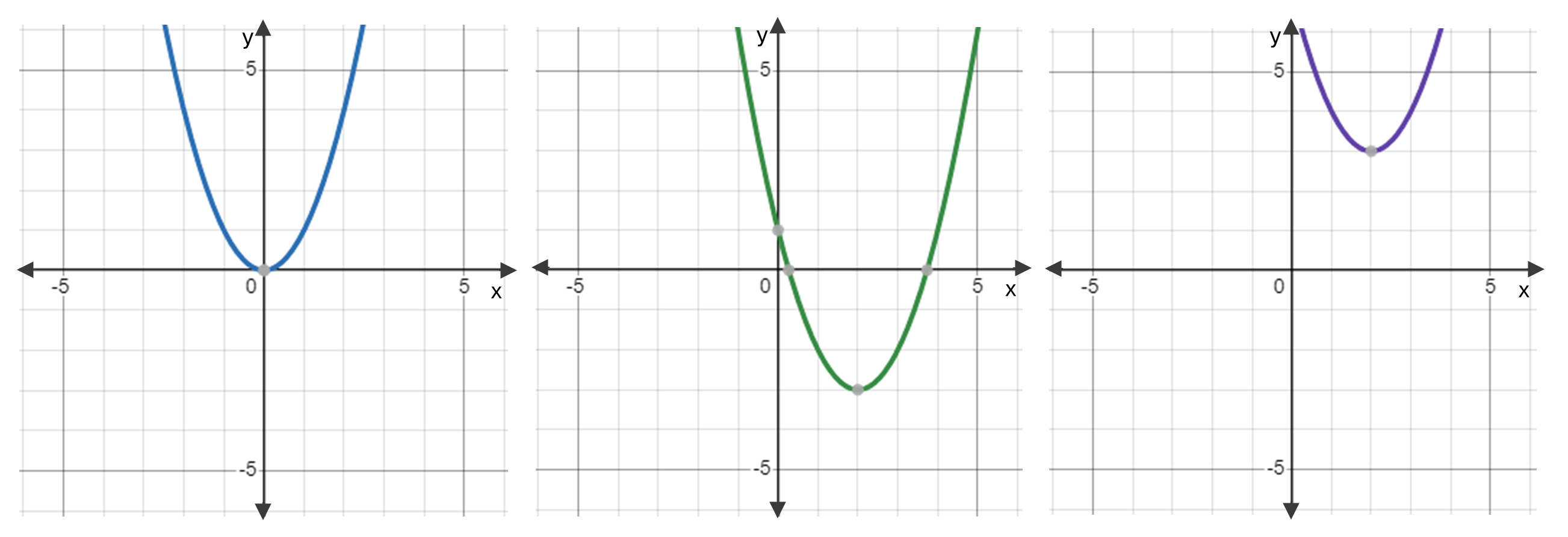
While this quadratic equation has only one solution, note that often there will be two solutions, and sometimes there will be no (real) solutions at all. To understand why this is the case, it can be helpful to look at the graphs of some quadratic equations. As seen below these take the form of parabolas, and the places at which these parabolas intersect the \(x\) (horizontal) axis are the solutions to the equation (as this is when the equation is equal to \(0\)).
The first image below is an example of where the parabola only intersects the \(x\) axis once, and hence there is only one solution. The second image is an example of where the parabola intersects the \(x\) axis twice, and hence there are two solutions. Finally, the third image is an example of where the parabola does not intersect the \(x\) axis at all, and hence there are no solutions.
There are various ways of solving quadratic equations, depending on the nature of the equation. This page outlines three different techniques.
Solving when \(b = 0\)
Probably the easiest type of quadratic equation to solve is one where \(b = 0\); i.e. when the equation is of the form:
\[ax^2 + c = 0\]You can solve equations like this as follows:
-
Rearrange the equation so that \(ax^2\) is by itself on the left hand side of the equation, by adding or subtracting the constant \(c\) from both sides, as applicable; like you would do for a linear equation.
-
Divide through both sides of the equation by \(a\) (assuming \(a \neq 1\)); like you would do for a linear equation.
- Take the square root of both sides of the equation, keeping in mind that this may result in either:
- no real solution, if you are taking the square root of a negative number (as there is no real number that can be squared to make a positive number);
- one solution of \(0\), if you are taking the square root of \(0\); or
- both a positive and a negative solution, if you are taking the square root of a positive number. For example, \(\sqrt{100} = \pm 10\) (“plus or minus ten”), as both \(10\) and \(-10\) are square roots of \(100\).
- Check that the answer(s) you have obtained is/are actually correct, by substituting the value back into the original equation and evaluating it. If it’s not correct, go back and see if you can find where you went wrong and work through the steps again.
Example: Solve the quadratic equation \(2x^2 - 72 = 0\)
Solution: Following the steps above, we have:
\[\begin{aligned} && 2x^2 - 72 &= 0 && \\\ \therefore && 2x^2 - 72 + 72 &= 0 + 72 && \textrm{ (undo subtraction by adding) } \\\ \therefore && 2x^2 &= 72 && \textrm{ (simplify) } \\\ \therefore && \frac{2x^2}{2} &= \frac{72}{2} && \textrm{ (divide both sides by 2) } \\\ \therefore && x^2 &= 36 && \textrm{ (simplify) } \\\ \therefore && \sqrt{x^2} &= \sqrt{36} && \textrm{ (take square root of both sides) } \\\ \therefore && x &= \pm 6 && \textrm{ (evaluate - equation is solved!) } \end{aligned}\]Finally, substituting \(\pm 6\) back into the original equation gives \(2(\pm 6)^2 - 72 = 2(36) - 72 = 72 - 72 = 0\) as required. So the solution is correct.
</div>
Once you have worked through the example above, have a go at using this technique to find the value of \(x\) in some or all of the following quadratic equations:
1. \(x^2 - 36 = 0\)
\[\begin{aligned} && x^2 - 36 &= 0 \\\ \therefore && x^2 - 36 + 36 &= 0 + 36 && \textrm{ (undo subtraction by adding) } \\\ \therefore && x^2 &= 36 && \textrm{ (simplify) } \\\ \therefore && \sqrt{x^2} &= \sqrt{36} && \textrm{ (take square root of both sides) } \\\ \therefore && x &= \pm6 && \textrm{ (simplify - equation is solved!) } \end{aligned}\]2. \(-x^2 + 100 = 0\)
\[\begin{aligned} && -x^2 + 100 &= 0 \\\ \therefore && -x^2 + 100 - 100 &= 0 - 100 && \textrm{ (undo addition by subtracting) } \\\ \therefore && -x^2 &= -100 && \textrm{ (simplify) } \\\ \therefore && \frac{-x^2}{-1} &= \frac{-100}{-1} && \textrm{ (undo multiplication by dividing) } \\\ \therefore && x^2 &= 100 && \textrm{ (simplify) } \\\ \therefore && \sqrt{x^2} &= \sqrt{100} && \textrm{ (take square root of both sides) } \\\ \therefore && x &= \pm10 && \textrm{ (simplify - equation is solved!) } \end{aligned}\]3. \(5x^2 + 30 = 0\)
\[\begin{aligned} && 5x^2 + 30 &= 0 \\\ \therefore && 5x^2 + 30 - 30 &= 0 - 30 && \textrm{ (undo addition by subtracting) } \\\ \therefore && 5x^2 &= -30 && \textrm{ (simplify) } \\\ \therefore && \frac{5x^2}{5} &= \frac{-30}{5} && \textrm{ (undo multiplication by dividing) } \\\ \therefore && x^2 &= -6 && \textrm{ (simplify) } \\\ \therefore && \sqrt{x^2} &= \sqrt{-6} && \textrm{ (take square root of both sides) } \\\ \therefore && x &\textrm{ has no real solutions } && \end{aligned}\]Solving by factorising
Another way you can solve a quadratic equation is by factorising the equation using two sets of brackets. This isn’t always easy or even possible, but if you notice that the equation can be relatively easily factorised, this can be a quick method of solving it. You can solve like this as follows:
-
Factorise the quadratic equation, as detailed in the Factorising section of this module.
-
In order for the quadratic equation to equal zero at least one of the factors must be zero, so you can solve it by setting each factor equal to zero and solving - like you would for a linear equation.
-
Check that the answer(s) you have obtained is/are actually correct, by substituting the value back into the original equation and evaluating it. If it’s not correct, go back and see if you can find where you went wrong and work through the steps again.
Example: Solve the quadratic equation \(x^2 + 7x + 12 = 0\)
Solution: Following the steps above, we have:
-
\(x^2 + 7x + 12 = 0\) can be factorised as \((x + 3)(x + 4)\)
-
Therefore either \(x + 3 = 0\), or \(x + 4 = 0\)
Solving \(x + 3 = 0\) gives \(x = -3\), while solving \(x + 4 = 0\) gives \(x = -4\)
Therefore the two solutions are \(x = -3\) and \(x = -4\) -
Substituting these values back into the original equation gives \((-3)^2 + 7(-3) + 12 = 9 - 21 + 12 = 0\) and \((-4)^2 + 7(-4) + 12 = 16 - 28 + 12 = 0\) as required.
</div>
Once you have worked through the example above, have a go at using this technique to find the value of \(x\) in some or all of the following quadratic equations:
1. \(x^2 + 7x + 6 = 0\)
Factorising gives \((x + 6)(x + 1) = 0\)
Therefore \(x + 6 = 0\), or \(x + 1 = 0\)
Solving these equations respectively gives two solutions: \(x = -6\) or \(x = -1\)
2. \(x^2 - 4x - 5 = 0\)
Factorising gives \((x + 1)(x - 5) = 0\)
Therefore \(x + 1 = 0\), or \(x - 5 = 0\)
Solving these equations respectively gives two solutions: \(x = -1\) or \(x = 5\)
3. \(x^2 + 3x = 0\)
Factorising gives \(x(x + 3) = 0\)
Therefore \(x = 0\), or \(x + 3 = 0\)
Solving gives two solutions: \(x = 0\) or \(x = -3\)
Solving using the quadratic formula
Finally, a way that you can solve any quadratic equation is using the quadratic formula. Note that this will not always be the quickest way to solve it, so it is a good idea to have a quick check and assess whether the previous two techniques will work first, but it is a method that works in all situations - and is sometimes the only method you will be able to use.
The quadratic formula states that for a quadratic equation \(ax^2 + bx + c = 0\), the value of \(x\) is given by:
\[x = \frac{-b \pm \sqrt{b^2 - 4ac}}{2a}\]Example: Solve the quadratic equation \(2x^2 + 3x - 10 = 0\)
Solution: Following the steps above, we have:
\[\begin{aligned} x &= \frac{-3 \pm \sqrt{3^2 - 4(2)(-10)}}{2(2)} \\\ &= \frac{-3 \pm \sqrt{9 + 80}}{4} \\\ &= \frac{-3 \pm \sqrt{89}}{4} \\\ &= \frac{-3 \pm 9.43}{4} \\\ &= \frac{6.43}{4} \textrm{ or } \frac{-12.43}{4} \\\ &= 1.61 \textrm{ or } -3.11 \end{aligned}\]Finally, substituting these values back into the original equation gives \(2(1.61)^2 + 3(1.61) - 10 \approx 0\) and \(2(-3.11)^2 + 3(-3.11) - 10 \approx 0\), as required.
</div>
Once you have worked through the example above, have a go at solving some or all of the following quadratic equations using one of the three techniques described above:
1. \(-x^2 + 10 = 0\)
\[\begin{aligned} && -x^2 + 10 &= 0 \\\ \therefore && -x^2 + 10 - 10 &= 0 - 10 && \textrm{ (undo addition by subtracting) } \\\ \therefore && -x^2 &= -10 && \textrm{ (simplify) } \\\ \therefore && \frac{-x^2}{-1} &= \frac{-10}{-1} && \textrm{ (undo multiplication by dividing) } \\\ \therefore && x^2 &= 10 && \textrm{ (simplify) } \\\ \therefore && \sqrt{x^2} &= \sqrt{10} && \textrm{ (take square root of both sides) } \\\ \therefore && x &= \pm3.16 && \textrm{ (simplify - equation is solved!) } \end{aligned}\]2. \(x^2 + 4x + 4 = 0\)
Factorising gives \((x + 2)^2 = 0\)
Therefore \(x + 2 = 0\)
Solving gives one solution: \(x = -2\)
3. \(4x^2 + 20 = 0\)
\[\begin{aligned} && 4x^2 + 20 &= 0 \\\ \therefore && 4x^2 + 20 - 20 &= 0 - 20 && \textrm{ (undo addition by subtracting) } \\\ \therefore && 4x^2 &= -20 && \textrm{ (simplify) } \\\ \therefore && \frac{4x^2}{4} &= \frac{-20}{4} && \textrm{ (undo multiplication by dividing) } \\\ \therefore && x^2 &= -5 && \textrm{ (simplify)} \\\ \therefore && \sqrt{x^2} &= \sqrt{-5} && \textrm{ (take square root of both sides)} \\\ \therefore && x &\textrm{ has no real solutions } && \end{aligned}\]4. \(x^2 + 4x - 12 = 0\)
Factorising gives \((x + 6)(x - 2) = 0\)
Therefore \(x + 6 = 0\) or \(x - 2 = 0\)
Solving these equations respectively gives two solutions: \(x = -6\) or \(x = 2\)
5. \(x^2 +2x - 10 = 0\)
\[\begin{aligned} x &= \frac{-2 \pm \sqrt{2^2 - 4(1)(-10)}}{2(1)} \\\ &= \frac{-2 \pm \sqrt{4 + 40}}{2} \\\ &= \frac{-2 \pm \sqrt{44}}{2} \\\ &= \frac{-2 \pm 6.63}{2} \\\ &= \frac{4.63}{2} \textrm{ or } \frac{-8.63}{2} \\\ &= 2.32 \textrm{ or } -4.32 \end{aligned}\]6. \(x^2 + 9x - 52 = 0\)
Factorising gives \((x + 13)(x - 4) = 0\)
Therefore \(x + 13 = 0\) or \(x - 4 = 0\)
Solving these equations respectively gives two solutions: \(x = -13\) or \(x = 4\)
Exponents & logarithms
This page introduces the concepts of exponents and logarithms, and details key laws that can be used when evaluating problems involving them.
In brief, it covers the following:
- The definition of an exponent
- How to evaluate problems involving exponents using the exponent laws
- The definition of a logarithm
- How to evaluate problems involving logarithms using the logarithm laws
</div>
What are exponents?
Exponents, otherwise known as indices or powers, are used as a shorthand notation for repeated multiplication. For example, \(5^4\) indicates that \(5\) needs to be multiplied by itself \(4\) times:
\[5^4 = 5 \times 5 \times 5 \times 5\]In this case we say that the number \(5\) is the base and the number \(4\) is the exponent or power. Some other examples of exponents, and how they are evaluated, are as follows:
Example 1: Evaluate \(3^2\)
Solution: \(3^2 = 3 \times 3 = 9\)
</div>
Example 2: Rewrite \(10 \times 10 \times 10 \times 10 \times 10 \times 2 \times 2\) using exponents.
Solution: Since \(10\) has been multiplied by itself \(5\) times and \(2\) has been multiplied by itself twice, we can rewrite this expression using exponents as \(10^5 \times 2^2\)
</div>
Once you have worked through the examples above, have a go at some or all of these problems involving exponents:
1. Evaluate \(8^3\)
\(8^ 3 = 8 \times 8 \times 8 = 512\)
2. Evaluate \(0^3\)
\(0^3 = 0 \times 0 \times 0 = 0\)
3. Evaluate \(10^9\)
\(10^9 = 10 \times 10 \times 10 \times 10 \times 10 \times 10 \times 10 \times 10 \times 10 = 1 000 000 000\)
4. Rewrite \(2 \times 2 \times 2 \times 2\) using exponents.
\(2^4\)
5. Rewrite \(5 \times 5 \times 5 \times 5 \times 5\) using exponents.
\(5^5\)
6. Rewrite \(3 \times 2 \times 2 \times 2 \times 2 \times 3\) using exponents.
\(3^2 \times 2^4\) (or \(2^4 \times 3^2\))
Exponent laws
There are various ‘laws’ that will make evaluating problems involving exponents much easier. Since these laws apply regardless of the value of the base and exponent, we will use variables when detailing them (the exception is that not all the laws apply when the base equals \(0\), so we will assume a non-zero base). In particular, the variables \(x\) and/or \(y\) will be used to represent non-zero bases, and the variables \(a\) and/or \(b\) will be used to represent exponents. For example:
\(x^a\) represents \(x\) being multiplied by itself \(a\) times
Now that we have defined our variables, let’s look at the exponents laws (while these are numbered here, note that there is no ‘set’ numbering system, and you may find them ordered differently in different places):
Law 1: \(x^1 = x\)
In other words, a base raised to the power of \(1\) is just equal to the value of the base.
Example: Use Law 1 to evaluate \(5^1\)
Solution: \(5^1 = 5\)
</div>
Law 2: \(x^0 = 1\)
In other words, a base raised to the power of \(0\) is just equal to \(1\).
Example: Use Law 2 to evaluate \(4^0\)
Solution: \(4^0 = 1\)
</div>
Law 3: \(x^ax^b = x^{a+b}\)
In other words, when you multiply two exponents with the same base you can rewrite it as a single exponent with the powers added together.
Example: Show how Law 3 works in order to evaluate \(2^32^4\)
Solution: \(2^32^4 = (2 \times 2 \times 2) \times (2 \times 2 \times 2 \times 2) = 2 \times 2 \times 2 \times 2 \times 2 \times 2 \times 2 = 2^7 (= 2^{3+4})\)
</div>
Law 4: \(\frac{x^a}{x^b} = x^{a-b}\)
In other words, when you divide two exponents with the same base you can rewrite it as a single exponent with the powers subtracted.
Example: Show how Law 4 works in order to evaluate \(\frac{10^5}{10^3}\)
Solution: \(\frac{10^5}{10^3} = \frac{10 \times 10 \times 10 \times 10 \times 10}{10 \times 10 \times 10} = 10 \times 10 = 10^2 (=10^{5-3})\)
</div>
Once you have worked through the examples above, have a go at using the exponent laws covered so far to evaluate some or all of the following:
1. Evaluate \(3^23^33^5\)
\(= 3^{2+3+5}\)
\(= 3^{10}\)
2. Evaluate \(\frac{5^35^4}{5^6}\)
\(= \frac{5^{3+4}}{5^6}\)
\(= \frac{5^7}{5^6}\)
\(= 5^{7-6}\)
\(= 5^1\)
\(= 5\)
3. Evaluate \(4^34^{-3}\)
\(= 4^{3+(-3)}\)
\(= 4^{3-3}\)
\(= 4^0\)
\(= 1\)
4. Evaluate \(2^32^2\)
\(= 2^{3+2}\)
\(= 2^5\)
5. Evaluate \(\frac{4^8}{4^5}\)
\(= 4^{8-5}\)
\(= 4^3\)
6. Evaluate \(\frac{5^45^2}{5^3}\)
\(= \frac{5^{4+2}}{5^3}\)
\(= \frac{5^6}{5^3}\)
\(= 5^{6-3}\)
\(= 5^3\)
Once you feel you have a handle on the first four exponent laws, have a look at these next four:
Law 5: \(x^{-a} = \frac{1}{x^a}\)
In other words, you can write negative exponents in two different ways: either using a negative exponent; or as \(1\) over the positive version of the exponent (i.e. as the reciprocal of the positive exponent). Both are correct, but sometimes one might be specified over the other, or sometimes writing it in a particular way will better help you simplify an expression or solve an equation.
Example 1: Use Law 5 to rewrite \(2^{-3}\) using a positive exponent.
Solution: \(2^{-3} = \frac{1}{2^3}\)
Example 2: Use Law 5 (and Law 1) to rewrite \(\frac{1}{4}\) using a negative exponent.
Solution: \(\frac{1}{4} = \frac{1}{4^1} = 4^{-1}\)
</div>
Law 6: \((x^a)^b = x^{ab}\)
In other words, any powers inside of brackets just need to be multiplied by any powers outside of brackets.
Example: Show how Law 6 works in order to evaluate \((2^2)^3\)
Solution: \((2^2)^3 = (2 \times 2)^3 = (2 \times 2) \times (2 \times 2) \times (2 \times 2) = 2 \times 2 \times 2 \times 2 \times 2 \times 2 = 2^6 (= 2^{2 \times 3})\)
</div>
Law 7: \((xy)^a = x^ay^a\)
In other words, when you multiply two (or more) exponents with the same power together, you can either write the bases inside brackets raised to a single power outside of the brackets, or you can write each of the exponents out separately. Again sometimes one way might be specified over the other, or sometimes writing it in a particular way will better help you simplify an expression or solve an equation.
Example: Show how Law 7 works in order to evaluate \((4 \times 5)^3\)
Solution: \((4 \times 5)^3 = (4 \times 5) \times (4 \times 5) \times (4 \times 5) = 4 \times 5 \times 4 \times 5 \times 4 \times 5 = 4 \times 4 \times 4 \times 5 \times 5 \times 5 = 4^35^3\)
</div>
Law 8: \((\frac{x}{y})^a = \frac{x^a}{y^a}\)
This is really just an extension of the previous law, and shows that if you have exponents with the same power divided by each other, again you may wish to have them raised to a single power outside of brackets, or to write each of the exponents out separately.
Example: Show how Law 8 works in order to evaluate \((\frac{4}{5})^3\)
Solution: \((\frac{4}{5})^3 = \frac{4}{5} \times \frac{4}{5} \times \frac{4}{5} = \frac{4 \times 4 \times 4}{5 \times 5 \times 5} = \frac{4^3}{5^3}\)
</div>
Once you have worked through the examples above, have a go at using the exponent laws covered so far to evaluate some or all of the following:
1. Evaluate \((5^{-2})^2\), giving your answer in terms of a positive exponent.
\(= 5^{-2 \times 2}\)
\(= 5^{-4}\)
\(= \frac{1}{5^4}\)
2. Evaluate \((3^{-4}4)^{-3}\), giving your answer in terms of positive exponents.
\(= (3^{-4})^{-3}4^{-3}\)
\(= (3^{-4 \times -3})4^{-3}\)
\(= 3^{12}4^{-3}\)
\(= \frac{3^{12}}{4^3}\)
3. Evaluate \((\frac{5}{6^{-2}})^3\), giving your answer in terms of positive exponents.
\(= \frac{5^3}{(6^{-2})^3}\)
\(= \frac{5^3}{6^{-2 \times 3}}\)
\(= \frac{5^3}{6^{-6}}\)
\(= 5^36^6\)
4. Evaluate \((10^{-3})^{-2}\)
\(= 10^{-3 \times -2}\)
\(= 10^6\)
5. Evaluate \((5^24^{-4})^5\), giving your answer in terms of positive exponents.
\(= (5^2)^5(4^{-4})^5\)
\(= 5^{2 \times 5}4^{-4 \times 5}\)
\(= 5^{10}4^{-20}\)
\(= \frac{5^{10}}{4^{20}}\)
6. Evaluate \((\frac{3^2}{4^{-3}})^{-5}\), giving your answer in terms of positive exponents.
\(= \frac{(3^2)^{-5}}{(4^{-3})^{-5}}\)
\(= \frac{3^{2 \times -5}}{4^{-3 \times -5}}\)
\(= \frac{3^{-10}}{4^{15}}\)
\(= \frac{1}{3^{10}4^{15}}\)
Once you feel you have a handle on the first eight exponent laws, have a look at these last two:
Law 9: \(x^{\frac{1}{a}} = \sqrt[a]{x}\)
In other words, when your power is a fraction with numerator (top number) \(1\) and denominator (bottom number) \(a\), you can either just have a fractional exponent, or you can instead write it as the \(a^{th}\) root of the base (the \(a^{th}\) root is just an extension of the square root, and is the number that when multiplied by itself \(a\) times will give the number inside the root; e.g. \(\sqrt[3]{8} = 2\), since \(2 \times 2 \times 2 = 8\)). Either is correct, but sometimes one way might be specified over the other, or sometimes writing it in a particular way will better help you simplify an expression or solve an equation.
Example 1: Use Law 9 to rewrite \(9^{\frac{1}{2}}\) as a root of the base.
Solution: \(9^{\frac{1}{2}} = \sqrt[2]{9} = \sqrt{9}\)
Example 2: Use Law 9 to rewrite \(\textrm{ }\sqrt[3]{27}\) as an exponent with a fractional power.
Solution: \(\sqrt[3]{27} = 27^{\frac{1}{3}}\)
</div>
Law 10: \(x^{\frac{b}{a}} = \sqrt[a]{x^b} =( \sqrt[a]{x})^b\)
This law is an extension of the previous law (and sometimes only this law might be specified), and says that when your power is a fraction with numerator (top number) \(b\) and denominator (bottom number) \(a\), you can either just have a fractional exponent, or you can instead write it as the \(a^{th}\) root of the base to the power of \(b\). Further, this power can be written in one of two ways; either inside the root sign or outside (try it yourself and check that they given the same value!). Any one of the three ways is correct, but sometimes one way might be specified over the other, or sometimes writing it in a particular way will better help you simplify an expression or solve an equation.
Example 1: Use Laws 6 and 9 to show how Law 10 works to evaluate \(8^{\frac{2}{3}}\) as a root of the base, with the power inside the root sign.
Solution: \(8^{\frac{2}{3}} = 8^{2 \times \frac{1}{3}} = (8^2)^{\frac{1}{3}} = \sqrt[3]{8^2}\)
Example 2: Use Laws 6 and 9 to show how Law 10 works to evaluate \(8^{\frac{2}{3}}\) as a root of the base, with the power outside the root sign.
Solution: \(8^{\frac{2}{3}} = 8^{\frac{1}{3} \times 2} = (8^{\frac{1}{3}})^2 = (\sqrt[3]{8})^2\)
</div>
Once you have worked through the examples above, have a go at using the exponent laws to evaluate some or all of the following:
1. Evaluate \(16^{\frac{1}{4}}\), by first converting the exponent to a root. Don’t forget you should end up with both a positive and negative answer!
\(= \sqrt[4]{16}\)
\(= \pm 2\)
2. Evaluate \(64^{\frac{1}{2}}\), by first converting the exponent to a root. Don’t forget you should end up with both a positive and negative answer!
\(= \sqrt[2]{64}\)
\(= \pm 8\)
3. Evaluate \(27^{\frac{5}{3}}\), by first converting the exponent to a root.
\(= (\sqrt[3]{27})^5\)
\(= 3^5\)
\(= 243\)
4. Evaluate \(8^{\frac{4}{3}}\), by first converting the exponent to a root.
\(= (\sqrt[3]{8})^4\)
\(= 2^4\)
\(= 16\)
What are logarithms?
Logarithms are the ‘opposite’ of exponents, in the same way as addition and subtraction are opposites and multiplication and division are opposites; that is, the two operations undo each other.
Logarithms also have bases, and the logarithm of a number with a certain base tells you how many times you need to multiply the base by itself in order to obtain that number. For example, evaluating \(\log_b{a}\) (‘the logarithm of \(a\) with base \(b\)’) tells you how many times you need to multiply \(b\) by itself in order to obtain \(a\) (note however that you can only have logarithms of positive numbers, and that only positive bases are typically useful, so we will only consider positive numbers when dealing with logarithms).
In order to evaluate a logarithm manually, you can perform repeated multiplication of the base until the correct answer is obtained.
Example: Evaluate \(\log_2{16}\)
Solution: To evaluate this you would determine how many times \(2\) needs to be multiplied by itself in order to equal \(16\). Repeated multiplication gives a solution of \(4\), since:
\[2 \times 2 \times 2 \times 2 = 2^4 = 16\]Therefore we have \(\log_2{16} = 4\), which tells us that the logarithm of \(16\) with base \(2\) is \(4\)
</div>
Since logarithms and exponents are opposite operations, it follows that one can be rearranged as the other, and you may have noticed this in the example above. In particular, if you have an equation that sets \(a\) equal to an exponent with base \(b\) and power \(c\) (where all three are positive numbers), it can be rearranged to an equation that sets \(c\) equal to the logarithm of \(a\) with base \(b\) (and vice versa):
\[a = b^c \Longleftrightarrow c = \log_b{a}\]This relationship means that logarithms can be used to solve for an unknown exponent in an exponential equation - which is one of the reasons you may need to use them.
Once you have worked through the above, have a go at some or all of these problems involving logarithms:
1. Evaluate \(\log_5{125}\)
\(5 \times 5 \times 5 = 5^3 = 125\)
So \(\log_5{125} = 3\)
2. Evaluate \(\log_4{1024}\)
\(4 \times 4 \times 4 \times 4 \times 4 = 4^5 = 1024\)
So \(\log_4{1024} = 5\)
3. Evaluate \(\log_3{243}\)
\(3 \times 3 \times 3 \times 3 \times 3 = 3^5 = 243\)
So \(\log_3{243} = 5\)
4. Evaluate \(\log_2{128}\)
\(2 \times 2 \times 2 \times 2 \times 2 \times 2 \times 2 = 2^7 = 128\)
So \(\log_2{128} = 7\)
5. Rearrange \(y = 5^x\) to give an equation for \(x\) in terms of a logarithm.
Rearranging gives \(x = \log_5{y}\)
6. Rearrange \(\log_3{x} = 5\) to give an equation for \(x\) in terms of an exponent, and hence solve for \(x\)
Rearranging gives \(x = 3^5\)
Hence \(x = 243\)
7. Rearrange \(\log_7{x} = 2\) to give an equation for \(x\) in terms of an exponent, and hence solve for \(x\)
Rearranging gives \(x = 7^2\)
Hence \(x = 49\)
While logarithms can have a range of different bases, as in the examples above, there are two bases that are used most commonly with logarithms - and there are buttons on a scientific calculator for evaluating these. The first of these bases is \(10\), and in fact if you see a logarithm written without any base at all you can usually assume the base to be \(10\). For example:
\[\log{100000} = \log_{10}{100000}\]The button for evaluating a log with base \(10\) on a scientific calculator is the ‘\(\log\)’ button.
Example: Evaluate \(\log{100000}\)
Solution: This logarithm can be evaluated on a calculator, for example by entering \(100000\) and then pressing ‘\(\log\)’ (although some calculators may require this in a different order). The result will be \(5\), indicating that \(\log{100000} = 5\)
</div>
The other commonly used base for logarithms is a special number known as Euler’s number, which is denoted by the letter \(e\). \(e\) is an irrational number that is very important in mathematics, economics and finance, and its first \(20\) digits are:
\[2.7182818284590452353…\]A logarithm with base \(e\) is referred to as a natural logarithm, and is generally denoted by \(\ln\). For example:
\[\ln{7.389} = \log_e{7.389}\]The button for evaluating a log with base \(e\) on a scientific calculator is the ‘\(\ln\)’ button.
Example: Evaluate \(\ln{7.389}\)
Solution: This logarithm can be evaluated on a calculator, for example by entering \(7.389\) and then pressing ‘\(\ln\)’ (although some calculators may require this in a different order). The result will be approximately \(2\), indicating that \(\ln{7.389} \approx 2\)
</div>
Once you have worked through the above, have a go at some or all of these problems involving evaluating logarithms on a calculator:
1. Evaluate \(\log{500}\)
Evaluating this logarithm using a calculator gives \(2.70\)
2. Evaluate \(\ln{200000}\)
Evaluating this logarithm using a calculator gives \(12.21\)
3. Evaluate \(\log{10000}\)
Evaluating this logarithm using a calculator gives \(4\)
4. Evaluate \(\ln{550}\), rounding to two decimal places
Evaluating this logarithm using a calculator gives \(6.31\)
5. Rearrange \(y = e^x\) to give an equation for \(x\) in terms of a natural logarithm
Rearranging gives \(x = \log_e{y} = \ln{y}\)
6. Rearrange \(400 = e^x\) to give an equation for \(x\) in terms of a natural logarithm, and hence solve for \(x\)
Rearranging gives \(x = \log_e{400} = \ln{400}\)
Hence \(x = 5.99\)
7. Rearrange \(\log{x} = 3\) to give an equation for \(x\) in terms of an exponent, and hence solve for \(x\)
Rearranging gives \(x = 10^3\)
Hence \(x = 1000\)
Lastly, note that you can also evaluate logarithms with bases other than \(10\) or \(e\) on a scientific calculator by first applying the change of base rule. This rule is as follows (where \(c\) is a positive number of your choosing; typically either \(10\) or \(e\)):
\[\log_b{a} = \frac{\log_c{a}}{\log_c{b}}\]Example: Evaluate \(\log_4{12}\) on a calculator by first applying the change of base rule.
Solution: Using the change of base rule to convert both logarithms to base \(10\) gives the following (note that you could also convert both logarithms to base \(e\), which would give the same result):
\[\begin{aligned} \log_4{12} &= \frac{\log_{10}{12}}{\log_{10}{4}} \\\ &= \frac{\log{12}}{\log{4}} \\\ &= \frac{1.079}{0.602} \\\ &= 1.792 \end{aligned}\]</div>
Once you have worked through the above, have a go at some or all of these problems involving applying the change of base rule in order to evaluate logarithms on a calculator:
1. Evaluate \(\log_6{20}\)
\[\begin{aligned} \log_6{20} &= \frac{\log_{10}{20}}{\log_{10}{6}} \\\ &= \frac{\log{20}}{\log{6}} \\\ &= \frac{1.301}{0.778} \\\ &= 1.672 \end{aligned}\]2. Evaluate \(\log_7{114}\)
\[\begin{aligned} \log_7{114} &= \frac{\log_{10}{114}}{\log_{10}{7}} \\\ &= \frac{\log{114}}{\log{7}} \\\ &= \frac{2.057}{0.845} \\\ &= 2.434 \end{aligned}\]3. Evaluate \(\log_5{200}\)
\[\begin{aligned} \log_5{200} &= \frac{\log_{10}{200}}{\log_{10}{5}} \\\ &= \frac{\log{200}}{\log{5}} \\\ &= \frac{2.301}{0.699} \\\ &= 3.292 \end{aligned}\]4. Evaluate \(\log_9{1500}\)
\[\begin{aligned} \log_9{1500} &= \frac{\log_{10}{1500}}{\log_{10}{9}} \\\ &= \frac{\log{1500}}{\log{9}} \\\ &= \frac{3.176}{0.954} \\\ &= 3.328 \end{aligned}\]5. Evaluate \(\log_3{2260}\)
\[\begin{aligned} \log_3{2260} &= \frac{\log_{10}{2260}}{\log_{10}{3}} \\\ &= \frac{\log{2260}}{\log{3}} \\\ &= \frac{3.354}{0.477} \\\ &= 7.030 \end{aligned}\]Logarithm laws
Just like with exponents, there are some ‘laws’ that will make evaluating problems involving logarithms much easier. Again we will use variables when detailing these, and note in particular that \(a\), \(b\) and \(c\) will be used to represent any positive numbers. The five most commonly used logarithm laws are as follows:
Law 1: \(\log_b{b} = 1\)
In other words, a logarithm of a number where the base equals that number is just equal to \(1\).
Example: Use Law 1 to evaluate \(\log_{10}{10}\)
Solution: \(\log_{10}{10} = 1\)
</div>
Law 2: \(\log_b{1} = 0\)
In other words, the logarithm of 1 is equal to zero, regardless of the base.
Example: Use Law 2 to evaluate \(\log_{10}{1}\)
Solution: \(\log_{10}{1} = 0\)
</div>
Law 3: \(\log_b{ac} = \log_b{a} + \log_b{c}\)
In other words, when two (or more) logarithms with the same base are added together, you can instead write it as a single logarithm with the same base and the values multiplied.
Example: Show how Law 3 works in order to evaluate \(\log_2{(4 \times 8)}\)
Solution: \(\log_2{(4 \times 8)} = \log_2{4} + \log_2{8}\textrm{ }[= 2 + 3 = 5 = \log_2{32}]\)
</div>
Law 4: \(\log_b{\frac{a}{c}} = \log_b{a} - \log_b{c}\)
In other words, when one logarithm is subtracted from another and they have the same base, you can instead write it as a single logarithm with the same base and the first value divided by the second.
Example: Show how Law 4 works in order to evaluate \(\log_2{\frac{64}{4}}\)
Solution: \(\log_2{\frac{64}{4}} = \log_2{64} - \log_2{4}\textrm{ }[= 6 - 2 = 4 = \log_2{16}]\)
</div>
Law 5: \(\log_b{a^c} = c \log_b{a}\)
In other words, when you have the logarithm of some number to a power, this is the same as the logarithm multiplied by that power.
Example: Show how Law 5 works in order to evaluate \(\log_2{8^2}\)
Solution: \(\log_2{8^2} = 2 \log_2{8}\textrm{ }[= 2(3) = 6 = \log_2{64}]\)
</div>
Once you have worked through the examples above, have a go at using the logarithm laws to evaluate some or all of the following:
1. Evaluate \(\log_{15}{15} + \log_3{3}\)
\(\log_{15}{15} + \log_3{3} = 1 + 1 = 2\)
2. Evaluate \(\log_{100}{100} + log_{15}{1}\)
\(\log_{100}{100} + log_{15}{1} = 1 + 0 = 1\)
3. Evaluate \(\log{(\frac{1}{100})}\)
\(\log{(\frac{1}{100})} = \log{1} - \log{100} = 0 - 2 = -2\)
4. Evaluate \(\log_6{4} + \log_6{54} + \log_7{1}\)
\(\log_{6}4 + \log_6{54} + 0 = \log_{6}4 + \log_6{54} = \log_{6}{(4 \times 54)} = \log_6{216} = 3\)
5. Evaluate \(2\log_8{2} + \log_8{128}\)
\(2\log_8{2} + \log_8{128} = \log_8{(2^2)} + \log_8{128} = \log_8{4} + \log_8{128} = \log_8{(4 \times 128)} = \log_8{512} = 3\)
6. Evaluate \(\log{10^5} - \log{10^2}\)
\(\log{(10^5)} - \log{(10^2)} = 5\log{10} - 2\log{10} = 5 - 2 = 3\)
7. Evaluate \(\log_2{40} + 3\log_2{6} - \log_2{270}\)
\(\log_2{40} + 3\log_2{6} - \log_2{270} = \log_2{40} + \log_2{(6^3)} - \log_2{270} = \log_2{40} + \log_2{216} - \log_2{270} = \log_2{(\frac{40 \times 216}{270})} = \log_2{32} = 5\)
Functions
This page introduces the concept of a function and details some common types, including linear, quadratic, exponential and logarithmic functions.
In brief, it covers the following:
- The definition of a function, and how to determine whether a relationship is a function
- Conventions for naming functions
- Some common types of functions
</div>
What is a function?
A function in mathematics is a relationship between input values and output values, whereby each input value has exactly one output value. This relationship can be visualised as follows:
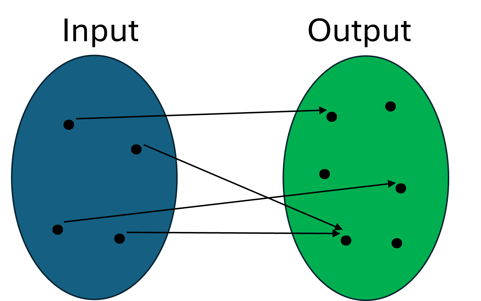
From this image, note that the set of input values is called the domain of the function, the set of all possible output values is called the codomain, and the set of output values that are actually mapped to by the input values is called the range.
Also note that while it is fine for multiple input values to be mapped to the same output value, as shown, one input value can not map to multiple output values as this violates the definition of a function.
As an example of a function, consider the linear relationship:
\[y = 2x + 3\]This function takes a number \(x\) and transforms it by multiplying it by \(2\) and adding \(3,\) in order to produce an output value called \(y.\) Some examples of these input and output values are as follows:
| Input value (x) | Output value (y) |
|---|---|
| -1 | 1 |
| 0 | 3 |
| 1 | 5 |
| 2 | 7 |
Note that the function \(y = 2x + 3\) works for all real numbers, but this is not always the case. Sometimes in order for a relationship to be a function, the domain and/or codomain needs to be restricted. For example, the relationship \(y = \sqrt{x}\) does not provide any (real) output values for negative input values, and it provides two output values for each positive input value (for example, the square root of \(9\) is both \(-3\) and \(3).\) Therefore, it is only a function if both the domain and codomain are limited to non-negative real numbers.
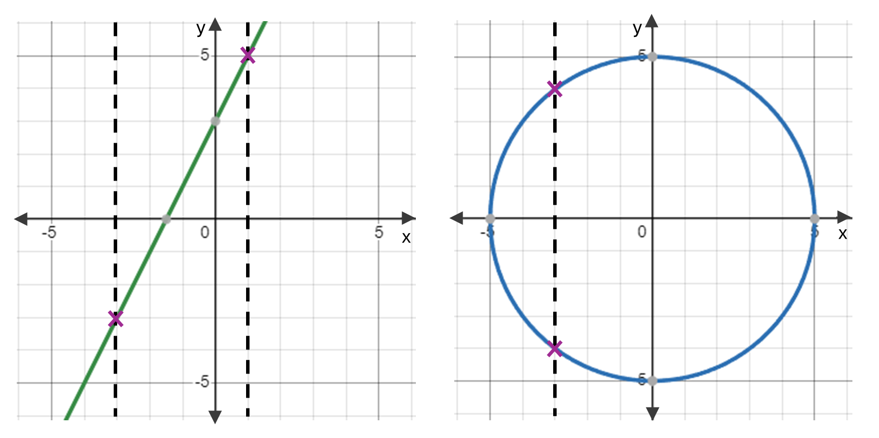
Note also that if you have a graph of a relationship, you can determine whether it is a function by performing the vertical line test. This test says that the relationship is a function if and only if each vertical line intersects the graph no more than once. For example, the relationship on the left (which is \(y = 2x + 3\)) is a function as it is not possible to draw a vertical line that intersects the graph more than once at any point. However, the relationship on the right is not a function as there is at least one point (in fact there are many) where a vertical line intersects the graph twice.
Check your understanding of functions by completing the following activity:
Function names
A function can just be stated in terms of \(x\) and \(y\) (or other variable names as relevant), as per the function \(y = 2x + 3\) stated previously. However, generally functions are given ‘names’, of which \(f\) is the most common. For example, the linear function \(y = 2x + 3\) could be written as:
\[f(x) = 2x + 3\]where:
- \(f\) is the name of the function, and we say \(f\) of \(x\) is equal to \(2x + 3\)
- \(x\) is the input value of the function.
If we had an input value of \(x = 2\) for this function, for example, then we could write the following (note this matches with the \(y\) value as shown in the table above):
\[f(2) = 7\]Check your understanding of function names by completing the following activity:
1. A function takes an input value \(z,\) squares it and then adds \(7.\) Write this as a function named \(f\)
\(f(z) = z^2 + 7\)
2. If \(f(x) = 3x - 5,\) find \(f(10)\)
\(f(10) = 25\)
Types of functions
There are many different types of functions, but here we will consider four types based on what has been covered in this module. These are as follows:
-
Linear functions: Linear equations in two variables are functions, and in particular they are linear functions. For example, \(f(x) = 2x + 3\) is a linear function.
-
Quadratic functions: Quadratic functions are of the form \(f(x) = ax^2 + bx + c, \) where \(a \neq 0.\) For example, \(f(x) = 2x^2 + 3x -2\) is a quadratic function.
-
Exponential functions: Exponential functions are of the form \(f(x) = a^x,\) where \(a > 0.\) For example, \(f(x) = 3^x\) is an exponential function.
-
Logarithmic functions: Logarithmic functions are of the form \(f(x) = \log_a{x},\) where \(a >0\) and \(a \neq 1.\) For example, \(f(x) = log_{10}{x}\) is a logarithmic function.
Check your understanding of different types of functions by completing the following activity:
1. \(g(x) = 10^x\) is what type of function?
This is an exponential function.
2. \(f(z) = z^2 + 3\) is what type of function?
This is a quadratic function.
Feedback
If you would like to provide feedback on this module please do so by answering some or all of the questions in the form below. Alternatively for any questions about the module please contact Library-UniSkills@curtin.edu.au
We review this feedback regularly, and take your suggestions on board to improve the module. Thank you for your feedback!
Explore more here
About UniSkills
UniSkills was created and is maintained by Curtin University Library. To report issues with UniSkills contact Library Help.
Twemoji icons by Twitter, Inc and other contributors, licensed under a CC-BY 4.0 licence.
Except where otherwise noted, UniSkills content in all it’s forms (website, PDFs etc) are licensed under a Creative Commons Attribution ShareAlike 4.0 International Licence. We ask that you attribute any use of the content as created by Curtin University Library with a link to the Library website.
This license does not extend to other Curtin University and Curtin University Library webpages, or to Curtin branding and trademarks. Curtin University’s copyright information is available on the Curtin website.