Introduction-to-Stata-printable-guide-UniSkills.pdf

Introduction to Stata

Table of Contents

Introduction

Welcome to the Introduction to Stata module. This module provides an introduction to using the statistical software Stata, which is installed on most computers at Curtin’s Australian campuses.

The module looks at some of the ways you can use the software to analyse quantitative data, and uses two small data sets as examples. The idea is that you can then apply these same concepts to any data of your own, regardless of your discipline or the amount of data you have. Note that if you are not familiar with some or all of the statistical concepts mentioned in this module, you may find it useful to work through the Introduction to statistics module first.

Your feedback on this module is very welcome and can be provided at any time on the feedback page, or alternatively for any questions about the module please contact Library-UniSkills@curtin.edu.au

What you will learn

How to create and use do-files and manage your working directory in Stata.
How to open a dataset, enter data and set up variables in Stata.
How to use Stata to calculate simple descriptive statistics.
How to use Stata to create simple graphs.
How to create new variables in Stata by performing transformations.
How to use Stata to test whether continuous variables are normally distributed.
How to obtain and interpret confidence intervals in Stata.
How to conduct t-tests and one-way ANOVA in Stata.
How to test for relationships between pairs of categorical and continuous variables using the chi-square test of independence and Pearson’s correlation (respectively) in Stata.<h2 id="digital-stata-getting-started">Getting started</h2>

When using Stata to help with your statistical analysis, it is highly likely that you will already have your data in some other electronic format. For example, in Excel or in an online survey tool such as Qualtrics. If this is the case you do not have to enter your data manually into Stata, and instead should just ensure that your variables are set up correctly. If you do not already have it in an electronic format though, you will need to enter the data as well as set up the variables. Either way, it is recommended that you write your commands in a do-file.

In brief, this page covers the following:

The key components of the Stata user interface
How to use Stata syntax to interact with the software, either by writing commands in the Command window or in a do-file
How to check and set your working directory
How to open an existing dataset in Stata, including by importing from other software
How to enter and save data in Stata
How to set up variables in Stata
How to save your dataset and results in Stata

The Stata user interface

When you open Stata you should see a user interface with four labelled windows; the History, Command, Variables, and Properties windows. In addition, the large window in the centre of the interface where the results are displayed is the Results window.

Click on the relevant part of the image below to learn more about each of these windows:

H5P interactive activity

In addition to the five windows displayed, you can also open the Data Editor and Do-file Editor windows:

The Data Editor window is used either to edit or browse the data in memory. To open it using the menu, you can select the Data tab, select Data Editor and then choose Data Editor (Edit) or Data Editor (Browse). Alternatively, you can type either the edit or browse commands in the Command window.
The Do-file Editor is used to create a do-file. You can open it using the menu by selecting the Window tab, selecting Do-file Editor and New Do-file Editor, or by typing the doedit command in the Command window.

Using Stata syntax

Although you can interact with Stata using the menus and dialog boxes, this module focuses on writing and using syntax - that is, entering and running commands. When doing this, some important things to keep in mind about the commands are as follows:

They are case sensitive, and need to be written all in lower case
They are written using American English spelling
You can use * or // to add single-line comments and /* */ to add multi-line comments as required

You can type your commands directly into the Command window, but a do-file enables you to keep a permanent record of everything you have done. In addition, it allows you to run multiple commands at once, to easily reproduce your results, and to share your workflow with others. To create one, open the Do-file Editor as detailed above, select File and Save as…, give the file an appropriate name and save it in a suitable location (for example, in your working directory). You can then write any commands in the do-file in the same way as you would in the Command window.

When you are ready to run the commands in your do-file, click the ‘Execute’ icon at the top of the screen (the image of a document with a play icon). Alternatively, you can also run it using the do command in the Command window as follows, replacing the name of the do-file with the appropriate name (and ensuring it is in your working directory - or changing the working directory or specifying the file path if not):

do "do-fileName.do"

Note that if you only want to run a certain command or commands in the do-file instead, rather than the whole thing, you can do so by highlighting the relevant line or lines and clicking the ‘Execute’ icon.

Managing your working directory

Your working directory is the default location for any files you read into or save in Stata. You can read and save files in locations other than your working directory, but you will need to specify the file path each time in this case.

You can check what your current working directory is by typing the pwd command in the Command window. If you find you need to change it you can use the cd command as follows, replacing the file path with the correct file path (note this does not need to be in the C drive):

cd "C:\Folder Name\Folder Name"

Note that if you are working with a do-file, as detailed above, it is recommended that you save it in your working directory. This way you should only need to set your working directory the first time you use the do-file, as after that Stata will automatically set the working directory to the location of the do-file when you open it directly (that is, by double clicking on the file to open it rather than opening Stata first). If you don’t open the do-file directly though, you will likely need to set your working directory each time (in which case, you may like to include the command to do this at the top of your do-file).

If you would like to create a new folder within your working directory you can do this using the mkdir command. For example, you could create a new folder within your working directory called Results, to save your results, as follows:

mkdir Results

Opening a dataset

To open an existing dataset in Stata, you can utilise the use command. Do so as follows, replacing the name of the dataset with the correct name (and ensuring it is in your working directory - or changing the working directory or specifying the file path if not):

use "datasetName.dta", clear

Note that the addition of the clear option in this command tells Stata to remove any data already in memory before loading the new dataset. Stata only allows one dataset at a time, so this helps avoid errors. You can also use clear on its own at any time to empty the memory.

If you wish to import data from another source (such as Excel, SPSS or SAS) you will need to use one of the commands below instead (again, after ensuring it is in your working directory or changing the working directory or specifying the file path if not).

Importing from Excel
You can import an Excel dataset using the following command, replacing the name of the Excel workbook with the correct name:

import excel "workbookName.xlsx"

In addition, you can add one or more of the below options after a comma to modify the behaviour of this command.

Option 1. Add the following to specify the name of a particular sheet to be imported, replacing the name of the sheet with the correct name (noting that this is only required when there is more than one sheet in the workbook, and the one you want to import is not the first one):

sheet("sheetName")

Option 2. Add the following to specify a particular range of cells to import, replacing the range of cells with the correct name (noting that this is only required when you do not want to import all of the data):

cellrange(A2:F20)

Option 3. Add the following to use the header row of the Excel spreadsheet as the variable names and labels in Stata:

firstrow

Importing from SPSS
You can import an SPSS dataset using the following command, replacing the name of the dataset with the correct name:

import spss "datasetName.sav"

Importing from SAS
You can import a SAS dataset using the following command, replacing the name of the dataset with the correct name:

import sas "datasetName.sad7bdat", bcat("value labels file")

Finally, if you wish to import data from an online survey tool such as Qualtrics, you will need to export it from the survey tool. While some tools may have the functionality to export to a Stata data file, Qualtrics does not, and therefore you will need to export it to an Excel file or SPSS file before importing as described.

Entering and saving data

If you don’t already have your data in an electronic format you can enter it directly in Stata instead. The data we will enter here has also been used for the examples in the next few pages of this module, and comes from the following simple survey:

SAMPLE QUESTIONNAIRE
Please complete this questionnaire by circling your response or by writing your answer on the line provided. Thank you for your co-operation in providing the information.

How old are you?________
Which gender do you identify as?

Male Female Non-binary Prefer not to say Prefer to self-describe:________
Do you have any children?

Yes No
What is your household’s average daily energy consumption (in kWh) in summer?________
What is your household’s average daily energy consumption (in kWh) in winter?________
How many people live in your household?________
Would you like to reduce your household’s energy consumption?

Strongly disagree Disagree Neutral Agree Strongly agree

Note that as each of these questions only allows for one response, there will be one variable per question and hence seven variables. However, any other variables which allow multiple responses will need to have one variable for each possible response.

To enter data for these seven variables, or any others, in Stata, you can use the input command. When you do this, you will need to specify a name for each of the variables. These should be representative of the data, and each one has to be unique. Whilst variable names can be anything you choose, there are some rules to follow:

The maximum number of characters in each name is 32
The characters can only be letters, numbers, or underscores (spaces or other characters are not allowed), and the first character cannot be a number
The variable names are case sensitive, so for example Age, age and AGE are all different variable names

For this example, and for any other data you enter, these names could be related to the questions (for example ‘Age’ for the first variable), they could be the question numbers (for example ‘Q1’; if you export data from Qualtrics the variable names will be the question numbers), or they could be anything else that makes sense to you. Here we will name the variables ‘age’, ‘gender’, ‘children’, ‘summer_consumption’, ‘winter_consumption’, ‘household_size’ and ‘consumption_reduction’.

We will enter the following data for 10 (fictional) individuals who completed the survey:

age	gender	children	summer_consumption	winter_consumption	household_size	consumption_reduction
21	1	2	17	18	2	4
35	1	1	26	22	4	5
29	2	1	25	28	5	3
46	3	1	19	20	3	4
32	2	2	12	13	1	2
25	2	2	16	18	2	4
41	2	1	26	27	6	2
	2	2	15	16	2	3
26	1	2	32	29	5	5
48	2	1	40	33	7	5

Remove clear command from below but mention it again to be used if required

To enter this data, and specify the variable names, type the following in the Command window. When you do this, note that the clear command clears any data that is already stored in memory, while the end command signifies that you have finished entering data. Furthermore, the . indicates that there is missing numeric data (for missing string data, use “” instead):

clear
input age gender children summer_consumption winter_consumption household_size consumption_reduction
21 1 2 17 18 2 4
35 1 1 26 22 4 5
29 2 1 25 28 5 3
46 3 1 19 20 3 4
32 2 2 12 13 1 2
25 2 2 16 18 2 4
41 2 1 26 27 6 2
. 2 2 15 16 2 3
26 1 2 32 29 5 5
48 2 1 40 33 7 5
end

Once you have done this, you should see the names of the variables appear in the Variables window at the top right of the screen. In addition, you can view or edit the data using the Data Editor window as required.

Setting up variables

Regardless of whether you import data from another source or enter it from scratch, you will need to make sure that your variables are set up correctly by specifying their properties. The following sections detail how to do this.

Naming variables

If you need to rename a variable or variables, you can do so using the rename command. To rename a single variable, follow this command with the name of the old variable and then the new variable. For example, to rename the ‘consumption_reduction’ variable to ‘Consumption_reduction’ (recalling that Stata is case sensitive) you would type the following:

rename consumption_reduction Consumption_reduction

To rename more than one variable at a time, follow the rename command with the names of the old and new variables in brackets instead. For example, to rename the ‘summer_consumption’, ‘winter_consumption’ and ‘household_size’ variables to ‘Summer_consumption’, ‘Winter_consumption’ and ‘Household_size’ respectively, type the following:

rename (summer_consumption winter_consumption household_size) (Summer_consumption Winter_consumption Household_size)

Alternatively, note that you can also change the case of variables by following the rename command with the old variable names and then either the upper (to change to all uppercase), lower (to change to all lowercase) or proper (to capitalise the first letter of each word) option after a comma. For example, to capitalise the first letter of the ‘age’, ‘gender’ and ‘children’ variables, type the following:

rename age gender children, proper

You should see the results of these variable name changes in the Variables window at the top right of the screen.

Assigning labels to variables

Because of the limit on the number of characters used in a variable name, the names can sometimes be rather cryptic. For example, the (newly renamed) ‘Summer_consumption’ and ‘Winter_consumption’ variables don’t provide the complete picture about the nature of the variables in the example above. Adding some extra labelling, though, can make all the difference. To add this extra information you can make use of the label variable command. For example, to add labels to these two variables type the following:

label variable Summer_consumption "Household energy consumption in kWh (summer)"
label variable Winter_consumption "Household energy consumption in kWh (winter)"

You should then see these labels next to the corresponding variable names in the Variables window at the top right of the screen.

Assigning labels to values for categorical variables

When entering data into Stata, the convention is to use numbers to represent categories for categorical data (visit the Data and variable types page of the Introduction to statistics module for more information on categorical data). This avoids any potential typos when entering category names, and makes the statistical analysis more straightforward. These numbers can be anything that make sense to you, but it is important that you let Stata know what category each number represents. You can do this by adding value labels for each categorical variable, which is a two-step process in Stata.

The first step requires using the label define command to define a value label set (that is, a list of the different numerical values to be used, and their corresponding category names). For example, you could define a value label set called ‘Gender_label’ (to be used with the ‘Gender’ variable in this example) as follows:

label define Gender_label 1 "Male" 2 "Female" 3 "Non-binary" 4 "Prefer not to say"

Once you have defined the value label set, you can apply it to a variable (or to multiple variables separately) using the label values command. For example, you can apply the ‘Gender_label’ set to the ‘Gender’ variable as follows:

label values Gender Gender_label

Once you have set up the value labels for the ‘Gender’ variable, do a similar thing for the other two categorical variables in this example (‘Children’ and ‘Consumption_reduction’) by running the following commands:

label define Children_label 1 "Yes" 2 "No"
label values Children Children_label
label define Consumption_reduction_label 1 "Strongly disagree" 2 "Disagree" 3 "Neutral" 4 "Agree" 5 "Strongly agree"
label values Consumption_reduction Consumption_reduction_label

Note that you can view the name of the value label set applied to each variable by selecting the name of the variable in the Variables window at the top right of the screen, and then viewing the variable properties in the Properties window at the bottom right of the screen. Or if preferred, you can use the ‘describe’ command as follows:

describe Gender

Either way, once you know the name of a variable label set you can use the label list command to view the values and corresponding labels for that set as required. For example:

label list Gender_label

Alternatively, you can just use the label list command with no variable label sets specified to list the details of all the label sets that have been created.

Setting the data type

Another important change to make for each variable is to tell the software what type of data it contains. For a numeric variable the default type is a float, but there are also four other options to choose from, namely byte, int, long and double. These types have the following properties:

Type	Stores	Minimum	Maximum	Bytes
byte	integers	\(-127\)	\(100\)	\(1\)
int	integers	\(-32 767\)	\(32 740\)	\(2\)
long	integers	\(-2 147 483 647\)	\(2 147 483 620\)	\(4\)
float	decimals (up to 7 digits)	\(-1.70141173319 \times 10^{38}\)	\(1.70141173319 \times 10^{38}\)	\(4\)
double	decimals (up to 16 digits)	\(-8.9884656743 \times 10^{307}\)	\(8.9884656743 \times 10^{307}\)	\(8\)

While the float type can continue to be used for all the variables in this dataset, it does use up additional unnecessary memory by allowing for larger numbers with decimal places. Therefore, you may wish to change some or all of the variables to type byte or int, which you can do with the recast command. For example, you can recast the ‘Gender’, ‘Children’, ‘Household_size’ and ‘Consumption_reduction’ variables to bytes and the ‘Age’, ‘Summer_consumption’ and ‘Winter_consumption’ variables to ints (just in case larger numbers are required) as follows:

recast byte Gender Children Household_size Consumption_reduction
recast int Age Summer_consumption Winter_consumption

Note that you can view the type of each variable by selecting the name of the variable in the Variables window at the top right of the screen, and then viewing the variable properties in the Properties window at the bottom right of the screen. Alternatively, you can use the describe command again.

Furthermore, note that string variables are stored as type str# (for example, str1, str10 or str50), where the number represents the maximum length of the string (alternatively, using strL allows for up to 2 000 000 000 characters). So you would specify this value as appropriate in the case of a string variable, again being mindful of using up unnecessary memory.

Formatting a variable

You can change how a variable is displayed, both in the Data Editor window and in output relating to that variable, using the format command. The default format is %9.0g, which indicates that:

the format is general numeric (that is, it automatically chooses between fixed and scientific notation as appropriate, and removes trailing zeros after the decimal point)
there are no commas in large numbers (for example 100000)
the field width is nine (that is, there are nine spaces reserved for displaying each value)

However, you can change this to:

be of a fixed numeric format (that is, a format that always shows numbers in standard decimal notation, and where you choose the number of decimal places), by replacing the g with an f
include commas in large numbers (for example 1,000,000), by adding a c on the end
adjust the field width, by changing the nine to a different value

In addition, if you are using a fixed numeric format you can also edit the number after the decimal place to indicate how many decimal places to include in the output (when using a general numeric format, this number refers to the number of significant figures instead, and it is usually kept at zero to allow Stata to decide how many is appropriate).

For example, the following command formats the ‘Summer_consumption’ and ‘Winter_consumption’ variables so that they have a fixed numeric format, with commas in large numbers, a field width of six and two decimal places:

format Summer_consumption Winter_consumption %6.2fc

Note that you can view the format of each variable by selecting the name of the variable in the Variables window at the top right of the screen, and then viewing the variable properties in the Properties window at the bottom right of the screen. Alternatively, you can use the describe command again.

Adding notes for a variable

Finally, you can also add additional notes for a variable using the notes command if you want to provide more details than that specified in a label. For example, you could use the following command to add a note to the ‘Consumption_reduction’ variable:

notes Consumption_reduction : "Participants were asked whether they would like to reduce their household's energy consumption."

To view the notes for this variable you can then use the notes command as follows:

notes Consumption_reduction

Alternatively, you can just use the notes command without any variable names to view all the notes in the dataset.

Saving

Once you have set up your dataset it can be saved using the save command (when you do this it will be automatically saved in your working directory, unless you specify a different file path):

save "datasetName.dta"

Note that if you have already saved the dataset and want to overwrite it, you will need to add the replace option after a comma in the above command.

If you would like to save your output (that is, the statistics, tables and messages that appear in the Results window) to a file called a log file, you can use the log command. You just need to ensure that you run this command before you obtain your results, either in the Command window or in your do-file. The following version of this command will save the results to a file called ‘results.log’ which is saved in the Results folder in the working directory (as created previously):

log using "Results/results.log", replace

Note that the addition of the replace option in this command tells Stata to overwrite an existing log file with the new output. If you want to add new results to the end of an existing log file instead, use the append option instead of replace.

Either way, if you do create a log file make sure to include a command to close it once you’re finished, as follows:

log close
```<h2 id="digital-stata-descriptive">Descriptive statistics</h2>

One of the first things you will likely be doing with your sample of data is analysing it using descriptive statistics. This page details some of the most common types of descriptive statistics you might need to use in Stata, organised according to the type of data (for more information on any of the descriptive statistics covered, visit the [Descriptive statistics](https://uniskills.library.curtin.edu.au/numeracy/statistics/descriptive) page of the _Introduction to statistics_ module).  

<div class="p-2 fillwithpad" style="background-color: #ededed !important; border: solid 2px #ededed !important; border-radius: 20px;" markdown="1">
In brief, this page covers how to use Stata to do the following:
* Analyse data for [one categorical variable](#digital-stata-descriptive-categorical-data---one-variable)
* Analyse data for [one continuous variable](#digital-stata-descriptive-continuous-data---one-variable)
* [Compare the mean](#digital-stata-descriptive-comparing-means) of a continuous variable between different categories 
* Establish whether there is an association between [two categorical variables](#digital-stata-descriptive-categorical-data---two-variables)
* Establish whether there is a linear relationship between [two continuous variables](#digital-stata-descriptive-continuous-data---two-variables)

</div>

Note that the examples covered here make use of the data described in the [Getting started](#digital-stata-getting-started) page of this module. If you want to work through the examples provided and haven't already created this dataset, you can download it using the link below: 

* {::nomarkdown}<i class="s-lg-file-icon fa fa-file-o" style="font-size:1.5em; margin-right:5px;"></i>{:/nomarkdown} [Stata sample data [DTA, 7kB]](https://uniskills.library.curtin.edu.au/assets/docs/Stata_sample_data.dta) 

Also note that if you wish to save any of the output obtained from these examples, or any other output, you can create a [log file](#digital-stata-getting-started-saving).

<h3 id="digital-stata-descriptive-categorical-data---one-variable">Categorical data - one variable</h3>

A question you may wish to ask of the sample data is: _How many respondents of each gender are there?_

Categorical variables such as the 'Gender' variable can be analysed in this way using a frequency distribution table. To obtain one, you can make use of the **tabulate** command (which you can shorten to **tab**), as follows:

tab Gender

Note that you can also add an option to include any missing values in this table (if you think it will be useful to treat the missing data as a category rather than excluding it from the frequency and percentage calculations), by adding **mi** after a comma at the end of the command.

Your output should appear in the Results window, and should look like the following:  

{::nomarkdown}<img class="img-fluid w-50 mx-auto" alt="A frequency table showing the categories of Male, Female and Non-binary, and with respective frequencies 3, 6 and 1, respective percentages 30%, 60% and 10%, and respective cumulative percentages 30%, 90% and 100%" src="/assets/images/Stata_frequency_output.PNG">{:/nomarkdown}  

The columns to the right of the column of category names in this frequency distribution table are as follows:

* **Freq.:** shows how many of the sample are in each category. For example, the sample consists of 3 males.
* **Percent:** shows what percentage of the sample are in each category. For example, 60% of the sample are female. 
* **Cum.:** gives the sum of all the percentages up to and including that row of the table. For example, 90% of the sample are either male or female.

<h3 id="digital-stata-descriptive-continuous-data---one-variable">Continuous data - one variable</h3>

A question you may wish to ask of the sample data is: _What is the mean age of the respondents?_   

To obtain descriptive statistics (including the mean) for a continuous variable such as the 'Age' variable, you can make use of the **summarize** command (which you can shorten to **sum**), as follows:

sum Age

Note that you can list multiple variables in this command, separated by a space, to obtain descriptive statistics for each as required. You can also add an option to include more statistics in the output (namely percentiles, variance, skewness and kurtosis), by adding **detail** after a comma at the end of the command.  

Your output should appear in the Results window, and should look like the following:

{::nomarkdown}<img class="img-fluid w-60 mx-auto" alt="Descriptive statistics for the Age variable, showing that there are 9 observations with a mean of 33.66667, standard deviation of 9.565563, minimum of 21 and maximum of 48" src="/assets/images/Stata_descriptives_output.PNG">{:/nomarkdown}  

While there is no single command in Stata to obtain the mode, if you would like to obtain this one option is to use the following commands:

preserve contract Age gsort -_freq list Age _freq if _freq == _freq[1] restore

<h3 id="digital-stata-descriptive-comparing-means">Comparing means</h3>

A question you may wish to ask of the sample data is: _How does the mean summer energy consumption of those with children compare to those without?_   

If you wish to compare the mean of a continuous variable (such as the 'Summer_consumption' variable) between different categories (such as for the 'Children' variable) you can do this using the **tabstat** command, as follows:

tabstat Summer_consumption, statistics(mean sd n) by(Children)

Your output should appear in the Results window, and should look like the following:  

{::nomarkdown}<img class="img-fluid w-40 mx-auto" alt="A table showing the mean, standard deviation and N values for the Summer_consumption variable, and for those who do and don't have children separately" src="/assets/images/Stata_compare_means.PNG">{:/nomarkdown}  

This output compares the mean, sample size and standard deviation for each category (although note you can include different statistics by adjusting the command as required). Based on this, we can see that the mean summer energy consumption of people with children in the sample is higher than the mean summer energy consumption of people without children.  

If you would like to learn how to test whether differences such as this are statistically and/or practically significant in terms of the population, visit the [Comparing means](#digital-stata-comparing-means-conducting-an-independent-samples-t-test) page of this module. 

<h3 id="digital-stata-descriptive-categorical-data---two-variables">Categorical data - two variables</h3>

A question you may wish to ask of the sample data is: _Is there an association between gender and desire to reduce energy consumption in the sample?_   

You can establish how many people of each gender there are in the sample, and how many people have different feelings about reducing energy consumption, using separate frequency distribution tables (as detailed in the [Categorical data - one variable](#digital-stata-descriptive-categorical-data---one-variable) section of this page). With frequency distribution tables for the two variables separately, though, it is not possible to find out how many of each gender have different feelings about reducing consumption. To do this you need a cross-tabulation (or contingency table) instead, with categories for the independent variable ('Gender') in the rows, and categories for the dependent variable ('Consumption_reduction') in the columns (you can learn more about independent and dependent variables in the [Data and variable types](https://uniskills.library.curtin.edu.au/numeracy/statistics/data-variable-types#independent-and-dependent-variables) page of the _Introduction to statistics_ module).   

To do this for the 'Gender' and 'Consumption_reduction' variables you can use the **tabulate** command again (which you can shorten to **tab**), this time with both variables, as follows:

tab Gender Consumption_reduction

Note again that you can include any missing values in this table by adding **mi** after a comma at the end of the command.

Your output should appear in the Results window, and should look like the following:

{::nomarkdown}<img class="img-fluid w-75 mx-auto" alt="A crosstabulation for the Gender and Consumption_reduction variables with frequencies only" src="/assets/images/Stata_gender_consumption_crosstabulation.PNG">{:/nomarkdown}  

From this table you can see the number of people who are in each combination of categories; for example, there were two males and one female who strongly agreed that they wanted to reduce their energy consumption.  

Usually in a report though it is not sufficient to just specify these frequencies, and percentages are used instead (or in addition). Stata can include these in the table too, by adding one or more options after a comma. In particular, you can add the **row** option to include percentages of the row total, the **column** option to include percentages of the column total, and the **cell** option to include percentages of the overall total. In addition, you can add the **expected** option to include expected frequencies

For example, the following command will include both row percentages and expected frequencies:

tab Gender Consumption_reduction, row expected

Your output should appear in the Results window, and should look like the following:  

{::nomarkdown}<img class="img-fluid w-75 mx-auto" alt="A crosstabulation for the Gender and Consumption_reduction variables with frequencies, row percentages and expected frequencies" src="/assets/images/Stata_gender_consumption_crosstabulation_row_expected.PNG">{:/nomarkdown}  

From this table you can see the percentage of people of each gender who have different levels of agreement. For example, the 2 males who strongly agree equates to 66.67% of males in the sample, while the 1 female who strongly agrees equates to 16.67% of females in the sample. Note that if you would prefer to show, for example, what percentage of those who strongly agree are male and female, you would need to include column percentages instead.

The other values that have been included in this table are the expected counts. These provide an indication of whether there is an association between the variables in the sample, and in particular the closer the expected and the actual frequencies are to each other, the less likely it is that there is an association between them (for more information on expected frequencies see the [Descriptive statistics](https://uniskills.library.curtin.edu.au/numeracy/statistics/descriptive#descriptive-statistics-for-two-categorical-variables) page of the _Introduction to statistics_ module). With such a small sample size in this example this is not really relevant, but if the current discrepancies continued with a larger sample (for example, over double the number of males who strongly agreed than expected) then it would provide an indication that there is some sort of association between gender and level of agreement.   

If you would like to learn how to test whether an association is statistically and/or practically significant in terms of the population, visit the [Assessing relationships](#digital-stata-assessing-relationships-testing-for-association) page of this module.

<h3 id="digital-stata-descriptive-continuous-data---two-variables">Continuous data - two variables</h3>

A question you may wish to ask of the sample data is: _Is there a linear relationship between summer and winter energy consumption in the sample?_   

Pearson's correlation coefficient can be used to establish the strength and direction of a linear relationship (or lack of) between two continuous variables in a sample, for example the 'Summer_consumption' and 'Winter_consumption' variables. You can do this using the **correlate** command, as follows:

correlate Summer_consumption Winter_consumption

Your output should appear in the Results window, and should look like the following:  

{::nomarkdown}<img class="img-fluid w-40 mx-auto" alt="" src="/assets/images/Stata_correlation_summer_winter_consumption.PNG">{:/nomarkdown}  

This table displays the correlation of each selected variable with every other selected variable (in this case there are only two, but note that more variables can be selected). This means that the diagonal just shows the correlation of each variable with itself, which can be ignored. The other value shows that Pearson's correlation coefficient for the 'Summer_consumption' and 'Winter_consumption' variables is .9524, indicating that there is a strong positive linear correlation between summer and winter energy consumption (for more information on correlation see the [Descriptive statistics](https://uniskills.library.curtin.edu.au/numeracy/statistics/descriptive#descriptive-statistics-for-two-continuous-variables) page of the _Introduction to statistics_ module).   

If you would like to learn how to test whether linear correlation is statistically and/or practically significant in terms of the population, visit the [Assessing relationships](#digital-stata-assessing-relationships-testing-for-linear-correlation) page of this module.<h2 id="digital-stata-graphs">Graphs</h2>

This page details how you can create and edit some simple graphs in Stata. For further information on selecting the right graphs to display data, or on how to interpret the different graphs, see the [Descriptive statistics](https://uniskills.library.curtin.edu.au/numeracy/statistics/descriptive) page of the _Introduction to Statistics_ module.

<div class="p-2 fillwithpad" style="background-color: #ededed !important; border: solid 2px #ededed !important; border-radius: 20px;" markdown="1">
In brief, this page covers how to do the following using commands in Stata:
- how to [create various graphs](#digital-stata-graphs-creating-graphs) using Stata commands
- how to [name and save](#digital-stata-graphs-naming-and-saving-graphs) your graphs in Stata
- how to [edit your graphs](#digital-stata-graphs-editing-graphs) using commands or the Graph Editor
</div>

Note that the examples covered here make use of the data described in the [Getting started](#digital-stata-getting-started) page of this module. If you want to work through the examples provided and haven't already created this dataset, you can download it using the link below: 

* {::nomarkdown}<i class="s-lg-file-icon fa fa-file-o" style="font-size:1.5em; margin-right:5px;"></i>{:/nomarkdown} [Stata sample data [DTA, 7kB]](https://uniskills.library.curtin.edu.au/assets/docs/Stata_sample_data.dta) 

Also note that if you wish to save any of the output obtained from these examples, or any other output, you can create a [log file](#digital-stata-getting-started-saving).

<h3 id="digital-stata-graphs-creating-graphs">Creating graphs</h3>

To create a **bar chart**, or bar graph, of one variable use the **graph** command as follows:

graph bar (count), over(Gender)

This will create a bar graph which will display in a separate Graph window. The chosen variable will be on the x-axis, and the frequency of each option will be on the y-axis as shown:  

{::nomarkdown}<img class="img-fluid w-60 mx-auto" alt="A bar graph showing the frequency values of the Gender variable options" src="/assets/images/stata_barchart.png">{:/nomarkdown}
  
To create a **histogram** of a continuous variable use the **histogram** command:

histogram Summer_consumption

{::nomarkdown}<img class="img-fluid w-60 mx-auto" alt="A histogram of the summer consumption variable." src="/assets/images/stata_histogram.png">{:/nomarkdown}
  
To create a **scatterplot** use the command **scatter** along with the two variables you wish to plot. Note that the variable to go on the y-axis should be written first, followed by the x-axis variable. For example, the following command produces the scatterplot shown:

scatter Winter_consumption Summer_consumption

{::nomarkdown}<img class="img-fluid w-60 mx-auto" alt="A scatterplot of the summer consumption vs winter consumption variables." src="/assets/images/Stata_scatterplot_summer_winter.png">{:/nomarkdown}
  
You can also add a line of best fit to your scatterplot by using the **twoway** command to overlay a line of best fit. When you do this, it is recommended to remove the legend so that it doesn't interfere with the graph width, as follows:

twoway scatter Winter_consumption Summer_consumption || lfit Winter_consumption Summer_consumption, legend(off)

{::nomarkdown}<img class="img-fluid w-60 mx-auto" alt="A scatterplot of the summer consumption vs winter consumption variables with a line of best fit." src="/assets/images/Stata_scatterplot_summer_winter_fit_line.png">{:/nomarkdown}
  
You may find that adding the line of best fit in this way means that the title no longer displays on the y-axis, as shown, but note you can fix this by adding an option to the command to [edit the title](#digital-stata-graphs-editing-graphs).
  
To create a **box-and-whisker plot** use the graph command with **box**:

graph box Summer_consumption

{::nomarkdown}<img class="img-fluid w-60 mx-auto" alt="A box and whisper plot of the summer consumption variable." src="/assets/images/stata_boxwhisper.png">{:/nomarkdown}
  
To create a **pie chart** use the graph command with **pie**:

graph pie, over(Gender)

{::nomarkdown}<img class="img-fluid w-60 mx-auto" alt="A pie chart for the gender variable." src="/assets/images/Stata_pie_chart.png">{:/nomarkdown}

<h3 id="digital-stata-graphs-naming-and-saving-graphs">Naming and saving graphs</h3>

When working with graphs in Stata, each new graph automatically replaces the previous one unless you name or save it. Naming a graph allows you to refer back to it later within the same session, while saving a graph creates a permanent file on your computer that you can reopen or use outside of Stata. You can do one or both of these as required.

To name the previously created bar chart, for example, you can make use of the **name** command. When doing this, adding **replace** means that any previous graph in the session with the same name will be overwritten. If you don't want this to happen you can omit it, however note that if you run the same command again it will produce an error message:

graph bar (count), over(Gender) name(barchart_gender, replace)

Once you have named your graph you can display it at a later time using the **graph display** command. For example:

graph display barchart_gender

When your graph is open in the Graph window, either immediately after you create it or after using the **graph display** command, you can export it using the **graph export** command. When you use this command you'll need to specify a name for the image file you're creating, which generally will be the same as the name you have already assigned it in Stata (if you have done this) but doesn't have to be. For example, the following command will export the previously created bar chart and will give it the same name as it was assigned in Stata:

graph export “barchart_gender.png”

Note that the graph exported using this command will automatically be saved in the [working directory](#digital-stata-getting-started-managing-your-working-directory), and that if you want it to be saved in a different location you will need to specify the file path as part of the command. If you want to create a new folder within your working directory to save your graphs you can do this, you will just need to [create the folder](-digital-stata-getting-started-managing-your-working-directory) first. For example, the following commands will save the bar chart in a new folder called Graphs:

mkdir Graphs graph export “Graphs/barchart_gender.png”

You can also save your graph using the **File > Save** option in the Graph window.

<h3 id="digital-stata-graphs-editing-graphs">Editing graphs</h3>

There a number of commands that allow you to edit your graphs. It is recommended that you name and save your graphs as you go so that it is easier for you to edit the graph you want to edit without having to retype all of your previous commands. 

You can add a title to your graph using the **title** command. For example, to give the bar graph the title _Gender of Participants_ we would use the following command (note the title is in brackets but also in quotation marks.):

graph barchart_gender title(“Gender of Participants”)

{::nomarkdown}<img class="img-fluid w-60 mx-auto" alt="A bar graph showing the frequency values of the Gender variable options. The graph has the title gender of Participants." src="/assets/images/stata_charts_title.png">{:/nomarkdown}
  
When adding a title to a histogram, a comma is required after the title command. For example:

histogram Summer_consumption, title(“Energy Consumption in Summer”)

You can also specify the names to be displayed on the x- and y-axes of your graph, this time using the **xtitle** and **ytitle** commands. For example, the following will add different axis titles to the previously created scatterplot with line of best fit:

twoway scatter Winter_consumption Summer_consumption || lfit Winter_consumption Summer_consumption, xtitle(“Energy consumption in summer”) ytitle(“Energy consumption in winter”) legend(off)

<h4 id="digital-stata-graphs-graph-editor">Graph editor</h4>

You can also use the **Graph Editor** to edit your graph. In the Graph window, click on _File_ and then _Start Graph Editor_. 

{::nomarkdown}<img class="img-fluid w-40 mx-auto" alt="An image of the File options with Start Graph Editor highlighted." src="/assets/images/stata_graph_editor.png">{:/nomarkdown}

You should now see a list of objects on the right hand side. If you can't see the list of objects, click on the small icon of a white box with blue lines.

{::nomarkdown}<img class="img-fluid w-60 mx-auto" alt="A small red circle is around the white box with blue line, showing that this will open the objects lists" src="/assets/images/stata_objects_list.png">{:/nomarkdown}

You can use this list to change the look of your graph, including adding titles to your axes. Click on the small plus sign next to each object option to see the changes you can make. For example, using our bar chart from earlier, clicking on the plus sign next to _scaleaxis_ (the vertical or $$y$$ axis) shows the option _title_. To change the title of this axis, double click on _title_, and enter the text into the text box. You can also make any other changes you'd like to make in this pop up, including the size and colour of the text, as well as the position of the text (in the **Format** tab). The _grpaxis_ or group axis refers to the horizontal or $$x$$ axis.

{::nomarkdown}<img class="img-fluid w-60 mx-auto" alt="The axis title change pop up box." src="/assets/images/stata_axis_titles_popup.png">{:/nomarkdown}

<h2 id="digital-stata-transformations">Transformations</h2>

Often when you are doing your analysis you will find that it is helpful to create new variables, or to make changes to existing variables. This page details three transformations which enable you to do this.

<div class="p-2 fillwithpad" style="background-color: #ededed !important; border: solid 2px #ededed !important; border-radius: 20px;" markdown="1">
In brief, this page covers the following:
* How to [compute a new variable](#digital-stata-transformations-computing-a-new-variable) using data from existing variables
* How to [recode a categorical variable](#digital-stata-transformations-recoding-categorical-variables) in order to create new categories for it
* How to [convert a string variable](#digital-stata-transformations-converting-a-string-variable) to a numeric variable
* How to [create categories for a continuous variable](#digital-stata-transformations-categorising-continuous-variables)
</div>

Note that the examples covered make use of the _Household energy consumption data.dta_ file, which contains fictitious data for 80 people based on a short 'Household energy consumption' questionnaire. If you want to work through the examples provided you can download the data file using the following link:

* {::nomarkdown}<i class="s-lg-file-icon fa fa-file-o" style="font-size:1.5em; margin-right:5px;"></i>{:/nomarkdown} [Household energy consumption data [DTA, 25kB]](https://uniskills.library.curtin.edu.au/assets/docs/Stata_Household_energy_consumption_data.dta) 

If you would like to read the sample questionnaire for which the data relates, you can do so using this link:

* {::nomarkdown}<i class="s-lg-file-icon fa fa-file-pdf-o" style="font-size:1.5em; margin-right:5px;"></i>{:/nomarkdown} [Household energy consumption questionnaire [PDF, 187kB]](https://uniskills.library.curtin.edu.au/assets/docs/SPSS_Household_energy_consumption_questionnaire_50098893.pdf)  

Also note that if you wish to save any of the output obtained from these examples, or any other output, you can create a [log file](#digital-stata-getting-started-saving).

<h3 id="digital-stata-transformations-computing-a-new-variable">Computing a new variable</h3>

Sometimes you may wish to create a new variable or variables to add to your data file, either from scratch or using the data from an existing variable or variables. For example, in the sample data file you may wish to create a new variable which gives the difference between summer and winter household energy consumption for each survey participant. You can do this using the **generate** command (which you can shorten to **gen**), specifying the name of the new variable and how it is to be calculated as follows:

gen Consumption_difference = q6 - q7

Once you have done this, you should see the name of the new variable appear in the Variables window at the top right of the screen. In addition, you can view or edit the data using the [Data Editor window](#digital-stata-getting-started-the-stata-user-interface), and can edit the variable properties using the instructions provided in the [Getting started](-digital-stata-getting-started-setting-up-variables) page of this module.

As another example of when you might want to compute a new variable, consider questions q9 through q12, which all relate to satisfaction with different aspects of the participants' electricity provider. As these questions all use the same rating system (measured on a scale of 1 to 5, with 1 indicating 'Very unsatisfied' and 5 indicating 'Very satisfied'), the four variables representing these questions can be combined to come up with an overall satisfaction score.

One way of doing this is by adding all the variables together to create a score out of 20, which can be done using the **gen** command as follows:

gen overall_satisfaction = q9 + q10 + q11 + q12

If you run the **tab** command on this new variable (as described in the [Descriptive statistics](#digital-stata-descriptive-categorical-data---one-variable) page of this module) you will see that there are only 78 satisfaction scores, whereas there are 80 cases in the data file. Looking at the actual data reveals why; the data in row 30 is missing for all four of the variables 'q9' to 'q12', and the data in row 31 is missing for variables 'q10' and 'q12'. Since the numeric expression shown above only calculates new values for those cases that have complete data, the new variable has not been computed for rows 30 and 31.

Sometimes this will be what you want, but other times you will require data for the new variable regardless of whether some of the data is missing or not. To do this requires you to use the **egen** and **row_total** commands instead, as follows:

egen overall_satisfaction2 = rowtotal(q9 q10 q11 q12)

You may also like to experiment with other formulas. For example, if you wanted to calculate an average overall satisfaction score instead you could also try using two different, similar commands:

* The command **gen average_satisfaction = (q9 + q10 + q11 + q12) / 4** will again have missing data for both rows 30 and 31.
* The command **egen average_satisfaction = rowmean(q9 q10 q11 q12)** will have missing data only for row 30. For row 31, the average will be calculated by dividing by 2 instead of 4, since there are only two variables with data.

Regardless of which formula you choose to use, the new variable can then be analysed in the usual way.

<h3 id="digital-stata-transformations-recoding-categorical-variables">Recoding categorical variables</h3>

Sometimes you may wish to recode an existing categorical variable, most likely to reduce the number of categories by combining existing ones together. For example, in the sample data file you may wish to recode the 'q8' variable to reduce the number of categories from the current five to three (particularly as there are so few people in each category, and no-one in the 'Strongly disagree' category). You can do this using the **recode** command, and you can also add the **generate** (or **gen**) option if you would like to keep the existing variable and create a new variable, rather than overwriting the existing variable. For example, you can keep the existing 'q8' variable and create a new one which combines the existing categories into three as follows:

recode q8 (1/2=1) (3=2) (4/5=3), gen(q8_recoded)

Once you have done this, you should see the name of the new variable appear in the Variables window at the top right of the screen. In addition, you can view or edit the data using the [Data Editor window](#digital-stata-getting-started-the-stata-user-interface), and can edit the variable properties using the instructions provided in the [Getting started](-digital-stata-getting-started-setting-up-variables) page of this module. In particular, you can assign labels to the new variable as follows:

label define q8_recoded_label 1 “Disagree” 2 “Neutral” 3 “Agree” label values q8_recoded q8_recoded_label

<h3 id="digital-stata-transformations-converting-a-string-variable">Converting a string variable</h3>

Although Stata does allow alphabetic/string information to be entered as part of the data file, the more in-depth statistical analysis procedures require numeric data only (even if those numbers are simply codes or values representing categories).   

At the questionnaire design stage it may be very difficult to anticipate the responses that will be given though, so creating a tick-box type question can be too complicated or restrictive. Hence allowing open-ended responses may be preferable instead, and the choice then is to either numerically code the data before keying it in, or to recode the responses once they have been entered into Stata. This section details how to do the latter, and uses the 'q13' variable in the sample data file as an example. This variable stores participant responses to the question:   

_What kind of hot water system do you use at your property?_   

The variable is a string variable, and running the **tab** command on it gives the following:

{::nomarkdown}<img class="img-fluid w-75 mx-auto" alt="A frequency table showing twelve different response options" src="/assets/images/Stata_q13_frequency_table.png">{:/nomarkdown}  

This output shows only five different types of hot water systems, but because of different spelling and terminology and different use of upper and lower case characters, twelve different responses are listed. To reduce this twelve down to the real five, the different categories need to be combined (that is, recoded).  

To complete the first part of this two-step process requires use of the **encode** command, as follows:

encode q13, gen(q13_num)

This produces a new variable called 'q13_num', where the responses have been assigned to categories numbered from 1 to 12 (using a value label set also called 'q13_num').  

The second step of the process is then to reduce these 12 categories to the 5 required ones, using the standard [recode](#digital-stata-transformations-recoding-categorical-variables) command. In this case, the existing and new categories could be as follows:

{: .table .table-bordered .w-50  style="word-wrap:normal; word-break:normal;"}
|---
|Existing category|New category|  
|:----------------|:-----------|
|1 (electric) |1 (Electric)|
|2 (electric) |1 (Electric)|
|3 (gas instant) |2 (Instantaneous gas)|
|4 (Gas instant) |2 (Instantaneous gas)|
|5 (Gas instantaneous) |2 (Instantaneous gas)|
|6 (gas storage) |3 (Gas storage)|
|7 (Gas storage) |3 (Gas storage)|
|8 (Heat pump) |4 (Heat pump)|
|9 (Hot water heat pump) |4 (Heat pump)|
|10 (solar) |5 (Solar)|
|11 (Solar) |5 (Solar)|
|12 (Solar hot water) |5 (Solar)|
|---


<h3 id="digital-stata-transformations-categorising-continuous-variables">Categorising continuous variables</h3>

Sometimes it is helpful to transform a continuous variable into a categorical variable, as this provides additional analysis options. For example, in the sample data file you may wish to transform the continuous 'q1' variable into categories, perhaps in order to make some comparisons for different age groups.   

One way to do this is using the **recode** command as described in the previous section. For example, to make and label categories for people aged under 20, aged 20 to 29, aged 30 to 39 and aged 40 and above, you could type the following:

recode q1 (min/19=1) (20/29=2) (30/39=3) (40/max=4), gen(q1_grouped) label define q1_grouped_label 1 “<= 19” 2 “20 - 29” 3 “30 - 39” 4 “40+” label values q1_grouped q1_grouped_label

If your data has decimal places, however, you will need to think carefully about how you create your categories in order to ensure that no data is left out of them. If using the **recode** command to do this, some things to consider are that the ranges specified in the command are inclusive at both ends (for example, 20/29 includes both 20 and 29), and that if there are overlapping ranges the value will be assigned to the first matching range - so you may need to reorder the ranges in the command to account for this. Alternatively, you may find it easier to use the **generate** (or **gen**) and **replace** commands together instead. For example, you could create and label a second version of the previous variable as follows:

gen q1_grouped2 = . replace q1_grouped2 = 1 if q1 < 20 replace q1_grouped2 = 2 if q1 >= 20 & q1 < 30 replace q1_grouped2 = 3 if q1 >= 30 & q1 < 40 replace q1_grouped2 = 4 if q1 >= 40 & q1 != . label define q1_grouped_label2 1 “Age < 20” 2 “20 <= Age < 30” 3 “30 <= Age < 40” 4 “Age >= 40” label values q1_grouped2 q1_grouped_label2

Once you have done this, you should see the name of the new variable(s) appear in the Variables window at the top right of the screen. In addition, you can view or edit the data using the [Data Editor window](#digital-stata-getting-started-the-stata-user-interface), and can edit the variable properties using the instructions provided in the [Getting started](-digital-stata-getting-started-setting-up-variables) page of this module.
<h2 id="digital-stata-normal-distribution">The normal distribution</h2>

Many of the statistics detailed in the [Inferential statistics](#digital-stata-inferential) page of this module rely on the assumption that continuous data approximates a normal distribution, or that the sample size is large enough that the sampling distribution of the mean approximates a normal distribution. This page details how to use Stata to test whether a continuous variable is normally distributed, while the [_Introduction to statistics_](https://uniskills.library.curtin.edu.au/numeracy/statistics/normal-distribution) module provides more information about what the normal distribution is and when testing for it is required.   

<div class="p-2 fillwithpad" style="background-color: #ededed !important; border: solid 2px #ededed !important; border-radius: 20px;" markdown="1">
In brief, this page covers how to do the following in Stata:
* Test whether the distribution of a continuous variable [approximates a normal distribution](#digital-stata-normal-distribution-testing-for-normality)
* [Transform a variable](#digital-stata-normal-distribution-transforming-variables) in order to try and make it better approximate a normal distribution
* Test for normality of a continuous variable for [two or more categories](#digital-stata-normal-distribution-testing-for-normality-in-two-or-more-groups) of a categorical variable

</div>

Note that the examples covered make use of the _Household energy consumption data.dta_ file, which contains fictitious data for 80 people based on a short 'Household energy consumption' questionnaire. If you want to work through the examples provided you can download the data file using the following link:

* {::nomarkdown}<i class="s-lg-file-icon fa fa-file-o" style="font-size:1.5em; margin-right:5px;"></i>{:/nomarkdown} [Household energy consumption data [DTA, 25kB]](https://uniskills.library.curtin.edu.au/assets/docs/Stata_Household_energy_consumption_data.dta) 

If you would like to read the sample questionnaire for which the data relates, you can do so using this link:

* {::nomarkdown}<i class="s-lg-file-icon fa fa-file-pdf-o" style="font-size:1.5em; margin-right:5px;"></i>{:/nomarkdown} [Household energy consumption questionnaire [PDF, 187kB]](https://uniskills.library.curtin.edu.au/assets/docs/SPSS_Household_energy_consumption_questionnaire_50098893.pdf)  

Also note that if you wish to save any of the output obtained from these examples, or any other output, you can create a [log file](#digital-stata-getting-started-saving).

<h3 id="digital-stata-normal-distribution-testing-for-normality">Testing for normality</h3>

As explained in the [_Introduction to statistics_](https://uniskills.library.curtin.edu.au/numeracy/statistics/normal-distribution) module, it is helpful to consult a number of different measures in order to make a decision about normality. You can use a series of commands in Stata to obtain the required output.

For example, to test whether the 'q6' variable (which measures average daily summer energy consumption in kWh in the sample data file) is normally distributed, run the following:

sum q6, detail swilk q6 histogram q6, normal name(histogram_q6, replace) stem q6 graph box q6, name(boxplot_q6, replace) qnorm q6, name(normalQQ_q6, replace)

The output should be as follows (use the **graph display** command to view the required graphs, as detailed in the [Graphs](#digital-stata-graphs-naming-and-saving-graphs) page of this module):

{::nomarkdown}<img class="img-fluid w-60 mx-auto" alt="Descriptive statistics for the q6 variable, showing a mean of 22.0125, median (50th percentile) of 22, skewness of 0.0482909 and kurtosis of 2.51102" src="/assets/images/Stata_normality_output_descriptive_statistics.png">{:/nomarkdown}   

{::nomarkdown}<img class="img-fluid w-60 mx-auto" alt="Shapiro Wilk output for the q6 variable, showing a p value of 0.73578" src="/assets/images/Stata_normality_output_Shapiro_Wilk.png">{:/nomarkdown}  

{::nomarkdown}<img class="img-fluid w-75 mx-auto" alt="Histogram output for the q6 variable, showing a roughly symmetrical histogram" src="/assets/images/Stata_normality_output_histogram.png">{:/nomarkdown}  

{::nomarkdown}<img class="img-fluid w-20 mx-auto" alt="Stem and leaf output for the q6 variable, showing a roughly symmetrical stem and leaf plot" src="/assets/images/Stata_normality_output_stem_and_leaf.png">{:/nomarkdown}  

{::nomarkdown}<img class="img-fluid w-75 mx-auto" alt="Box plot for the q6 variable, showing a roughly symmetrical box plot with no outliers" src="/assets/images/Stata_normality_output_boxplot.png">{:/nomarkdown}  

{::nomarkdown}<img class="img-fluid w-75 mx-auto" alt="Normal QQ plot for the q6 variable, showing points that lie close to the diagonal line" src="/assets/images/Stata_normality_output_normalQQ.png">{:/nomarkdown}  

This output can then be evaluated as explained in the [_Introduction to statistics_](https://uniskills.library.curtin.edu.au/numeracy/statistics/normal-distribution) module. In particular, you should observe the following:  

* The mean and median (as shown in the first table) are extremely similar. Note that if you would also like to compare the mode, you can obtain this as detailed in the [Descriptive statistics](#digital-stata-descriptive-continuous-data---one-variable) page of this module. While this is a bit higher, at \\(25\\), this is less of a concern.

* The skewness is \\(0.048\\) (as shown in the first table), which is well within the acceptable range of \\(-1\\) to \\(1\\)  

* The kurtosis is \\(2.51\\) (as shown in the first table), which is within the acceptable range of \\(2\\) to \\(4\\) (note that Stata provides the value for actual kurtosis, rather than excess kurtosis, which ideally should be 3 but can be anywhere within this range)

* The \\(p\\) value for the Shapiro-Wilk test is \\(.736\\) (as listed under 'Prob>z' in the second table), which is greater than \\(.05\\) as required.

* The histogram is roughly symmetrical.

* The stem and leaf plot is roughly symmetrical.

* The points do not deviate much from the line in the Normal Q-Q plot.

* The median is approximately in the middle of the box plot, the whiskers are of similar length and there are no outliers.

Hence it can be concluded that the 'q6' variable is approximately normally distributed.

<h3 id="digital-stata-normal-distribution-transforming-variables">Transforming variables</h3>

If you find that a variable is not normally distributed when you require it to be, you can try transforming the variable to see if this makes it better approximate a normal distribution. Some examples of transformations to try are provided in the [_Introduction to statistics_](https://uniskills.library.curtin.edu.au/numeracy/statistics/normal-distribution#transforming-variables) module.   

You can apply any of these transformations by generating a new variable using the **gen** command, as described in the [Transformations](#digital-stata-transformations-computing-a-new-variable) page of this module. Once you have done this, you will need to test again for normality in the usual way.

<h3 id="digital-stata-normal-distribution-testing-for-normality-in-two-or-more-groups">Testing for normality in two or more groups</h3>

Sometimes rather than testing that all of a continuous variable's data is normally distributed, you need to check that the continuous variable's data is normally distributed for each category of a categorical variable. In future you may want to write a [loop](https://www.stata.com/manuals/pforeach.pdf) in Stata to do this, but in the meantime probably the easiest option is to adapt the previous normality commands to filter for each category manually.

For example, to test whether the 'q6' variable (which measures average daily summer energy consumption in kWh in the sample data file) is normally distributed for each group of the 'q3' variable (which shows whether or not the participant has any children in the sample data file), you should first establish the category numbers used. One way of doing this is as follows:

tab q3, nolabel

The output from this command should be as follows:

{::nomarkdown}<img class="img-fluid w-50 mx-auto" alt="A table showing frequencies, percentages and cumulative percentages for two categories, numbered 1 and 2" src="/assets/images/Stata_category_numbers.png">{:/nomarkdown}  

Next, you can use these category numbers to run the normality commands for each category separately, as follows:

sum q6 if q3 == 1, detail swilk q6 if q3 == 1 histogram q6 if q3 == 1, normal name(histogram_q6_q3_1, replace) stem q6 if q3 == 1 graph box q6 if q3 == 1, name(boxplot_q6_q3_1, replace) qnorm q6 if q3 == 1, name(normalQQ_q6_q3_1, replace)

sum q6 if q3 == 2, detail swilk q6 if q3 == 2 histogram q6 if q3 == 2, normal name(histogram_q6_q3_2, replace) stem q6 if q3 == 2 graph box q6 if q3 == 2, name(boxplot_q6_q3_2, replace) qnorm q6 if q3 == 2, name(normalQQ_q6_q3_2, replace)

The output will be very similar to the output obtained without filtering, but this time there will be a set of statistics and graphs for each group. These should be analysed separately, and you may sometimes find that the data is normally distributed for all groups, for some groups only, or for none of the groups. In this case, the output indicates that the 'q6' variable is normally distributed for both the group that has children, and the group that doesn't.<h2 id="digital-stata-inferential">Inferential statistics</h2>

There are two key types of inferential statistics, estimation and hypothesis testing, and Stata can be used to assist with both. This page looks at confidence intervals and at the fundamentals of hypothesis testing with regards to Stata, while subsequent pages of the module focus on how to conduct some common inferential statistical tests in Stata. Alternatively, for more information on inferential statistics you may like to visit the [_Introduction to statistics_](https://uniskills.library.curtin.edu.au/numeracy/statistics/inferential) module.  

<div class="p-2 fillwithpad" style="background-color: #ededed !important; border: solid 2px #ededed !important; border-radius: 20px;" markdown="1">
In brief, this page covers the following:
* How to [calculate a confidence interval](#digital-stata-inferential-determining-a-confidence-interval) in Stata
* The steps involved in [hypothesis testing](#digital-stata-inferential-hypothesis-testing), and where Stata can assist
</div>

Note that the examples covered make use of the _Household energy consumption data.dta_ file, which contains fictitious data for 80 people based on a short 'Household energy consumption' questionnaire. If you want to work through the examples provided you can download the data file using the following link:

* {::nomarkdown}<i class="s-lg-file-icon fa fa-file-o" style="font-size:1.5em; margin-right:5px;"></i>{:/nomarkdown} [Household energy consumption data [DTA, 25kB]](https://uniskills.library.curtin.edu.au/assets/docs/Stata_Household_energy_consumption_data.dta) 

If you would like to read the sample questionnaire for which the data relates, you can do so using this link:

* {::nomarkdown}<i class="s-lg-file-icon fa fa-file-pdf-o" style="font-size:1.5em; margin-right:5px;"></i>{:/nomarkdown} [Household energy consumption questionnaire [PDF, 187kB]](https://uniskills.library.curtin.edu.au/assets/docs/SPSS_Household_energy_consumption_questionnaire_50098893.pdf)  

Also note that if you wish to save any of the output obtained from these examples, or any other output, you can create a [log file](#digital-stata-getting-started-saving).

<h3 id="digital-stata-inferential-determining-a-confidence-interval">Determining a confidence interval</h3>

A **confidence interval** is a range of probable values for an unknown population parameter, based on the sample statistic (for example the mean). The percentage associated with the confidence interval is termed the **confidence coefficient**, and this is the level of confidence you have that the range actually includes the true value. Stata automatically calculates confidence intervals for a range of statistics, with the default being a \\(95\%\\) confidence interval. For example, the following details how to obtain and interpret a \\(95\%\\) confidence interval for the mean of a continuous variable. If you would like more information on confidence intervals you may first like to visit the [_Introduction to statistics_](https://uniskills.library.curtin.edu.au/numeracy/statistics/inferential#estimation) module.   

A question you may wish to ask of the data is: _Based on the data observed in the sample, what is the \\(95\%\\) confidence interval for the population mean summer energy consumption?_   

Before calculating this confidence interval in Stata, it is important to note that some assumptions need to be met when using a confidence interval to estimate the mean of a population. These assumptions are as follows:   

* **Assumption 1:** The sample is a random sample that is representative of the population.   

* **Assumption 2:** The observations are independent, meaning that measurements for one subject have no bearing on any other subject's measurements.   

* **Assumption 3:** The variable is normally distributed, or the sample size is large enough that the sampling distribution of the mean approximates a normal distribution. 

While these first two assumptions should be met during the design and data collection phases, the third assumption should be checked at this stage. For instructions on testing for normality in Stata, see the [The normal distribution](#digital-stata-normal-distribution) page of this module.   

If all assumptions are met (as is the case for this example), you can obtain a \\(95\%\\) confidence interval for the mean in Stata by using the **mean** command as follows:

mean q6

The output should be as follows: 

{::nomarkdown}<img class="img-fluid w-50 mx-auto" alt="A table showing the mean, its standard error and the confidence interval. The mean is 22.0125, the standard error is .7884638, and the confidence interval is 20.4431 to 23.5819" src="/assets/images/Stata_confidence_interval_mean.png">{:/nomarkdown}  

This tells us that based on what has been observed in the sample, we can be \\(95\%\\) confident that the mean summer energy consumption of the wider population is somewhere between \\(20.44\\) kWh (lower bound) and \\(23.58\\) kWh (upper bound).   

Note that to calculate a confidence interval for the mean with a confidence coefficient other than \\(95\%\\), you can add the **level** option after a comma with the required confidence coefficient in brackets. For example:

mean q6, level(99)

<h3 id="digital-stata-inferential-hypothesis-testing">Hypothesis testing</h3>

**Hypothesis testing** involves testing statements (hypotheses) about the population using data collected in the sample. The particular test to use depends on the nature of the hypothesis, and there are often versions of each test that are **parametric** (assume normal distribution and require at least one continuous variable) and **non-parametric** (don't assume normal distribution and can be used for ordinal variables). If you would like more information on hypothesis testing, you may like to visit the [_Introduction to statistics_](https://uniskills.library.curtin.edu.au/numeracy/statistics/inferential#hypothesis-testing) module.   

Some common examples of hypothesis tests are [one sample](#digital-stata-comparing-means-conducting-a-one-sample-t-test), [paired samples](-digital-stata-comparing-means-conducting-a-paired-samples-t-test) and [independent samples](#digital-stata-comparing-means-conducting-an-independent-samples-t-test) \\(t\\) tests, [one-way ANOVA](-digital-stata-comparing-means-conducting-an-one-way-anova), the [chi-square test of independence](#digital-stata-assessing-relationships-testing-for-association) and [Pearson's correlation](-digital-stata-assessing-relationships-testing-for-linear-correlation) (all of which are covered in later pages of this module). Whichever test you are using, it is important to note that conducting the test in Stata is just part of the process. In particular, the recommended steps to follow in order to successfully conduct a hypothesis test are listed below.

1. Determine the hypothesis to be tested.
2. Establish the appropriate test for the hypothesis.
3. Check that all assumptions for the test are valid (Stata can help with some of these).
4. Use Stata to conduct the relevant test and determine the \\(p\\) value and confidence interval (if applicable).
5. Interpret the result.

Examples of how to do this for each of the tests in the table are covered in the following pages.<h2 id="digital-stata-comparing-means">Comparing means</h2>

One of the reasons you may wish to do a hypothesis test is to determine whether there is a statistically significant difference between means, either for a single sample (in which case you would compare to a constant value) or for multiple independent or related samples (in which case you would compare between these different samples). Depending on the exact nature of the analysis, different tests are required, and this page details the process for performing some of the most common ones using Stata.

<div class="p-2 fillwithpad" style="background-color: #ededed !important; border: solid 2px #ededed !important; border-radius: 20px;" markdown="1">
In brief, it covers how to do the following in Stata:
* Conduct and interpret the output for a [one sample \\(t\\) test](#digital-stata-comparing-means-conducting-a-one-sample-t-test)
* Conduct and interpret the output for a [paired samples \\(t\\) test](#digital-stata-comparing-means-conducting-a-paired-samples-t-test)
* Conduct and interpret the output for an [independent samples \\(t\\) test](#digital-stata-comparing-means-conducting-an-independent-samples-t-test)
* Conduct and interpret the output for a [one-way ANOVA](#digital-stata-comparing-means-conducting-a-one-way-anova)
</div>

Note that the examples covered make use of the _Household energy consumption data.dta_ file, which contains fictitious data for 80 people based on a short 'Household energy consumption' questionnaire. If you want to work through the examples provided you can download the data file using the following link:

* {::nomarkdown}<i class="s-lg-file-icon fa fa-file-o" style="font-size:1.5em; margin-right:5px;"></i>{:/nomarkdown} [Household energy consumption data [DTA, 25kB]](https://uniskills.library.curtin.edu.au/assets/docs/Stata_Household_energy_consumption_data.dta) 

If you would like to read the sample questionnaire for which the data relates, you can do so using this link:

* {::nomarkdown}<i class="s-lg-file-icon fa fa-file-pdf-o" style="font-size:1.5em; margin-right:5px;"></i>{:/nomarkdown} [Household energy consumption questionnaire [PDF, 187kB]](https://uniskills.library.curtin.edu.au/assets/docs/SPSS_Household_energy_consumption_questionnaire_50098893.pdf)  

Also note that if you wish to save any of the output obtained from these examples, or any other output, you can create a [log file](#digital-stata-getting-started-saving).

<h3 id="digital-stata-comparing-means-conducting-a-one-sample-t-test">Conducting a one sample \\(t\\) test</h3>

A question you may wish to ask of the wider population is: _Does this sample come from a population where the mean summer daily energy consumption is \\(19\\)kWh_   

This question can be answered by following the [recommended steps](#digital-stata-inferential-hypothesis-testing), as follows:   

1. The appropriate hypotheses for this question are:  
\\(\textrm{H}\_\textrm{0}\\): The sample comes from a population with a mean summer daily energy consumption of \\(19\\)kWh  
\\(\textrm{H}\_\textrm{A}\\): The sample does not come from a population with a mean summer daily energy consumption of \\(19\\)kWh  

2. The appropriate test to use is the one sample \\(t\\) test, as we are testing whether the sample comes from a population with a specific mean (\\(19\\)kWh in this case). 

3. The assumptions for a one sample \\(t\\) test are as follows: 
* **Assumption 1:** The sample is a random sample that is representative of the population.   
* **Assumption 2:** The observations are independent, meaning that measurements for one subject have no bearing on any other subject's measurements.   
* **Assumption 3:** The variable is continuous.   
* **Assumption 4:** The variable is normally distributed, or the sample size is large enough to ensure normality of the sampling distribution. 

   While the first three assumptions should be met during the design and data collection phases, the fourth assumption should be checked at this stage (for instructions on doing this in Stata, see the [The normal distribution](#digital-stata-normal-distribution) page of this module). If the normality assumption is not met you can try transforming the data or conducting the One sample Wilcoxon signed-rank test instead (you can also use this test if you have an ordinal rather than continuous variable).  

4. If all the assumptions are met you can conduct the one sample \\(t\\) test in Stata using the **ttest** command as follows:

ttest q6 == 19

   The output should look like this: 

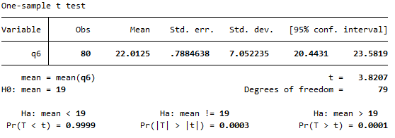   ![Output showing a mean of 22.0125, a p value of 0.0003 and confidence interval of 20.4431 to 23.5819](/assets/images/Stata_one_sample_t_test.png){:class="img-fluid w-70 mx-auto"}  

5. From the table we can see that the mean summer daily energy consumption in our sample is \\(22.01\\)kWh, which is \\(3.01\\)kWh more than our hypothesised value. To test whether this is a statistically significant difference, we need to refer to the \\(p\\) value and confidence interval.   

   While there are actually three \\(p\\) values listed below the table, the standard one to use is the middle one, which is the two-tailed \\(p\\) value. This is used to test for a difference in either direction (that is, to test whether the mean is significantly greater than or less than \\(19\\), as per our alternative hypothesis). Since \\(p < .05\\) (in fact \\(p = 0.0003\\)) and since the \\(95\%\\) confidence interval for the population mean summer daily energy consumption does not include the value of \\(19\\) (\\(95\% \textrm{CI}\\) [\\(20.4431\\)kWh, \\(23.5819\\)kWh]), we can reject the null hypothesis and conclude that the sample actually comes from a population with mean summer daily energy consumption significantly more than \\(19\\)kWh.   

   For more information on how to interpret these results see the [_Introduction to statistics_](https://uniskills.library.curtin.edu.au/numeracy/statistics/inferential#one-sample-t-test) module. 

<h3 id="digital-stata-comparing-means-conducting-a-paired-samples-t-test">Conducting a paired samples \\(t\\) test</h3>

A question you may wish to ask of the wider population is: _Is there a statistically significant difference between mean summer daily energy consumption and mean winter daily energy consumption?_   

This question can be answered by following the [recommended steps](#digital-stata-inferential-hypothesis-testing), as follows:   

1. The appropriate hypotheses for this question are:  
\\(\textrm{H}\_\textrm{0}\\): There is no significant difference between mean summer and winter daily energy consumption  
\\(\textrm{H}\_\textrm{A}\\): There is a significant difference between mean summer and winter daily energy consumption  

2. The appropriate test to use is the paired samples \\(t\\) test, as we are comparing the means of two related groups (summer and winter consumption for the sample people). 

3. The assumptions for a paired samples \\(t\\) test are as follows:   
* **Assumption 1:** The sample is a random sample that is representative of the population.   
* **Assumption 2:** The observations are independent, meaning that measurements for one subject have no bearing on any other subject's measurements.   
* **Assumption 3:** The variables are both continuous.   
* **Assumption 4:** Both variables as well as the difference variable (the differences between each data pair) are normally distributed, or the sample size is large enough to ensure normality of the sampling distributions. 

   While the first three assumptions should be met during the design and data collection phases, the fourth assumption should be checked at this stage (for instructions on doing this in Stata, see the [The normal distribution](#digital-stata-normal-distribution) and [Transformations](-digital-stata-transformations) pages of this module). If the normality assumption is not met you can try transforming the data or conducting the Wilcoxon signed rank test instead. You can also use this test if you have ordinal rather than continuous variables.   

4. If all the assumptions are met you can conduct the paired samples \\(t\\) test in Stata in Stata using the **ttest** command as follows:
 

ttest q6 == q7

   The output should look like this: 

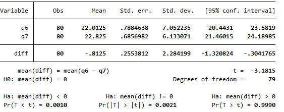   ![Output showing a mean difference of -0.8125, a p value of 0.0021 and confidence interval for the difference of -1.320824 to -0.3041765](/assets/images/Stata_paired_samples_t_test.png){:class="img-fluid w-70 mx-auto"}  

5. From the table we can see that the mean summer daily energy consumption in our sample is \\(22.01\\)kWh, while the mean winter daily energy consumption is \\(22.83\\)kWh; a difference of \\(0.81\\)kWh. To test whether this is a statistically significant difference, we need to refer to the \\(p\\) value and confidence interval.   

   While there are actually three \\(p\\) values listed below the table, the standard one to use is the middle one, which is the two-tailed \\(p\\) value. This is used to test for a difference in either direction (that is, to test whether one mean is significantly greater than or less than the other, as per our alternative hypothesis). Since \\(p < .05\\) (in fact \\(p= .0021\\)) and since the \\(95\%\\) confidence interval for the difference between the population mean summer and winter daily energy consumptions does not include zero (\\(95\% \textrm{CI}\\) [\\(-1.321\\)kWh, \\(-0.304\\)kWh]), we can reject the null hypothesis and conclude that the mean summer daily energy consumption is significantly less than the mean winter daily energy consumption.   

   For more information on how to interpret these results see the [_Introduction to statistics_](https://uniskills.library.curtin.edu.au/numeracy/statistics/inferential#paired-samples-t-test) module. 

<h3 id="digital-stata-comparing-means-conducting-an-independent-samples-t-test">Conducting an independent samples \\(t\\) test</h3>

A question you may wish to ask of the wider population is: _Is there a statistically significant difference in mean summer daily energy consumption for those with and without children?_   

This question can be answered by following the [recommended steps](#digital-stata-inferential-hypothesis-testing), as follows:   

1. The appropriate hypotheses for this question are:  
\\(\textrm{H}\_\textrm{0}\\): There is no significant difference in mean summer daily energy consumption for those with and without children  
\\(\textrm{H}\_\textrm{A}\\): There is a significant difference in mean summer daily energy consumption for those with and without children  

2. The appropriate test to use an independent samples \\(t\\) test, as we are comparing the means of two unrelated groups (summer consumption of those with and without children). 

3. The assumptions for an independent samples \\(t\\) test are as follows:   
* **Assumption 1:** The sample is a random sample that is representative of the population.   
* **Assumption 2:** The observations are independent, meaning that measurements for one subject have no bearing on any other subject's measurements.   
* **Assumption 3:** The dependent variable is continuous.   
* **Assumption 4:** The variable is normally distributed for both groups, or the sample size is large enough to ensure normality of the sampling distribution. 

   While the first three assumptions should be met during the design and data collection phases, the fourth assumption should be checked at this stage (for instructions on doing this in Stata, see the [The normal distribution](#digital-stata-normal-distribution) page of this module). If the normality assumption is not met you can try transforming the data or conducting the Mann-Whitney U test instead. You can also use this test if you have an ordinal rather than continuous dependent variable.   

4. If all the assumptions are met you can conduct the independent samples \\(t\\) test in Stata. However, first you may want to run Levene's Test for Equality of Variances to check whether the group variances are equal. You can do this using the **robvar** command, as follows:

robvar q6, by(q3)

   The output should look like this: 

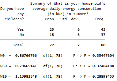   ![Output showing a p value for Levene's test of 0.354](/assets/images/Stata_Levenes_test.png){:class="img-fluid w-50 mx-auto"}  

   The \\(p\\) value for Levene's Test for Equality of Variances (listed in the first row below the table, after \\(Pr > F =\\)) is \\(p > .05\\) (in fact \\(p = .354\\)), so we can assume equal variances. In this case you would run the independent samples \\(t\\) test using the **ttest** command as follows (note that if the variances were not equal, you would add **unequal** directly after this command):

ttest q6, by(q3)

   The output should look like this: 

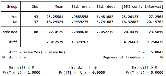   ![Output showing a mean difference of 7.012571, a p value of 0.0000 and confidence interval for the difference of 4.26667 to 9.758472](/assets/images/Stata_independent_samples_t_test.png){:class="img-fluid w-70 mx-auto"}  

5. From the table we can see that the mean summer daily energy consumption in our sample for those with children is \\(25.26\\)kWh, while for those without children it is \\(18.24\\)kWh; a difference of \\(7.01\\)kWh. To test whether this is a statistically significant difference, we need to refer to the \\(p\\) value and confidence interval.   

    While there are actually three \\(p\\) values listed below the table, the standard one to use is the middle one, which is the two-tailed \\(p\\) value. This is used to test for a difference in either direction (that is, to test whether one mean is significantly greater than or less than the other, as per our alternative hypothesis). Since \\(p < .05\\) (in fact \\(p= .0000\\), which doesn't mean that \\(p\\) is actually zero but that it is very very small) and since the \\(95\%\\) confidence interval for the difference between the population mean summer daily energy consumptions of those with and without children does not include zero (\\(95\% \textrm{CI}\\) [\\(4.267\\)kWh, \\(9.758\\)kWh]), we can reject the null hypothesis and conclude that the mean summer daily energy consumption is significantly more for those with children compared to those without.   

   For more information on how to interpret these results see the [_Introduction to statistics_](https://uniskills.library.curtin.edu.au/numeracy/statistics/inferential#independent-samples-t-test) module. 

<h3 id="digital-stata-comparing-means-conducting-a-one-way-anova">Conducting a one-way ANOVA</h3>

A question you may wish to ask of the wider population is: _Is there a statistically significant difference in mean summer daily energy consumption for any of the different marital statuses?_   

This question can be answered by following the [recommended steps](#digital-stata-inferential-hypothesis-testing), as follows:   

1. The appropriate hypotheses for this question are:  
\\(\textrm{H}\_\textrm{0}\\): There is no significant difference in mean summer daily energy consumption for any of the different marital statuses  
\\(\textrm{H}\_\textrm{A}\\): The mean summer daily energy consumption of at least one of the marital status groups is significantly different from the others  

2. The appropriate test to use a one-way ANOVA, as we are comparing the means of three unrelated groups (summer consumption of those with a marital status of single, married and other). 

3. The assumptions for a one-way ANOVA are as follows:   
* **Assumption 1:** The sample is a random sample that is representative of the population.   
* **Assumption 2:** The observations are independent, meaning that measurements for one subject have no bearing on any other subject's measurements.   
* **Assumption 3:** The dependent variable is continuous.   
* **Assumption 4:** The variable is normally distributed for each of the groups, or the sample size is large enough to ensure normality of the sampling distribution.   
* **Assumption 5:** The populations being compared have equal variances. 

   While the first three assumptions should be met during the design and data collection phases, the fourth and fifth assumptions should be checked at this stage For instructions on checking the normality assumption in Stata, see the [The normal distribution](#digital-stata-normal-distribution) page of this module. If this assumption is not met you can try transforming the data or conducting the Kruskall-Wallis one-way ANOVA instead. You can also use this test if you have an ordinal rather than continuous dependent variable.  
   
   To check the equal variances assumption you can run Levene's Test for Equality of Variances using the **robvar** command, as follows:
 

robvar q6, by(q4)

   The output should look like this: 

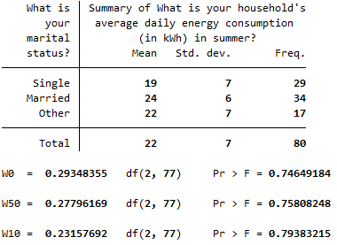   ![Output showing a p value for Levene's test of 0.74649184](/assets/images/Stata_ANOVA_Levenes_test.png){:class="img-fluid w-50 mx-auto"} 

   The \\(p\\) value for Levene's Test for Equality of Variances (listed in the first row below the table, after \\(Pr > F =\\)) is \\(p > .05\\) (in fact \\(p = .746\\)), so we can assume equal variances in this case. If the equal variances assumption is violated you will need to use a Welch or Brown-Forsythe statistic instead.   

4. If all the assumptions are met you can conduct the one-way ANOVA in Stata. You can do this using the **anova** command, which you may like to combine with the **tabstat** command (to obtain a table of descriptive statistics as part of the output) as follows:

tabstat q6, by(q4) stats (mean sd n) anova q6 q4

   The output should look like this: 

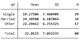      ![Output showing a sample mean summer energy consumption for single people of 19.27586, a sample mean for married people of 24.20588 and a sample mean for people in the other category of 22.29412](/assets/images/Stata_ANOVA_descriptives_table.png){:class="img-fluid w-40 mx-auto"}  

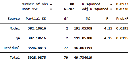      ![Output showing a p value for the one-way ANOVA of 0.0195](/assets/images/Stata_ANOVA_output.png){:class="img-fluid w-60 mx-auto"} 

5. From the descriptive statistics table we can see that the mean summer daily energy consumption in our sample for those who are single is \\(19.28\\)kWh, for those who are married it is \\(24.21\\)kWh and for those who classified their marital status as 'Other' it is \\(22.29\\)kWh. To test whether there are any statistically significant differences between these values, we need to refer to the ANOVA table and to the \\(p\\) value. Since \\(p < .05\\) (in fact \\(p = .0195\\)) we can reject the null hypothesis and conclude that the mean summer daily energy consumption is significantly different for at least one of the marital status groups.   

   To find out where the significant difference(s) lie you can conduct a post hoc test. While there are many different options to choose from, a common test to try is Tukey's HSD test. To obtain output for this you can run the **pwcompare** command as follows:

pwcompare q4, mcompare(tukey)

   The output should be as shown:

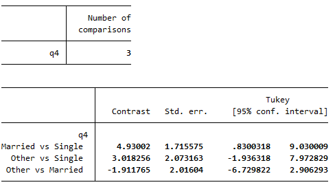   ![](/assets/images/Stata_post_hoc.png){:class="img-fluid w-70 mx-auto"}  

   From this table we can observe that the only significant difference in mean summer daily energy consumption is between the married and single groups. This is shown by the fact that the confidence interval for the difference in mean energy consumption between married and single people is the only confidence interval that does not contain the null value of zero.<h2 id="digital-stata-assessing-relationships">Assessing relationships</h2>

Hypothesis testing is often used to assess whether a statistically significant relationship exists between two or more variables. The type of test you use depends on the nature of those variables.

<div class="p-2 fillwithpad" style="background-color: #ededed !important; border: solid 2px #ededed !important; border-radius: 20px;" markdown="1">
In brief, this page covers how to do the following in Stata:
* Conduct and interpret the output for a [chi-square test of independence](#digital-stata-assessing-relationships-testing-for-association)
* Conduct and interpret the output for a [test of linear correlation](#digital-stata-assessing-relationships-testing-for-linear-correlation)
</div>

Note that the examples covered make use of the _Household energy consumption data.dta_ file, which contains fictitious data for 80 people based on a short 'Household energy consumption' questionnaire. If you want to work through the examples provided you can download the data file using the following link:

* {::nomarkdown}<i class="s-lg-file-icon fa fa-file-o" style="font-size:1.5em; margin-right:5px;"></i>{:/nomarkdown} [Household energy consumption data [DTA, 25kB]](https://uniskills.library.curtin.edu.au/assets/docs/Stata_Household_energy_consumption_data.dta) 

If you would like to read the sample questionnaire for which the data relates, you can do so using this link:

* {::nomarkdown}<i class="s-lg-file-icon fa fa-file-pdf-o" style="font-size:1.5em; margin-right:5px;"></i>{:/nomarkdown} [Household energy consumption questionnaire [PDF, 187kB]](https://uniskills.library.curtin.edu.au/assets/docs/SPSS_Household_energy_consumption_questionnaire_50098893.pdf)  

Also note that if you wish to save any of the output obtained from these examples, or any other output, you can create a [log file](#digital-stata-getting-started-saving).

<h3 id="digital-stata-assessing-relationships-testing-for-association">Testing for association</h3>

A question you may wish to ask of the wider population is: _Is there a statistically significant association between having children and owning a dishwasher?_   

This question can be answered by following the [recommended steps](#digital-stata-inferential-hypothesis-testing), as follows:   

1. The appropriate hypotheses for this question are:  
\\(\textrm{H}\_\textrm{0}\\): There is no significant association between having children and owning a dishwasher  
\\(\textrm{H}\_\textrm{A}\\): There is significant association between having children and owning a dishwasher  

2. The appropriate test to use is a chi-square test of independence, as we are testing for association between two categorical variables (having children and owning a dishwasher). 

3. The assumptions for the chi-square test of independence are as follows:   
* **Assumption 1:** The sample is a random sample that is representative of the population.   
* **Assumption 2:** The observations are independent, meaning that measurements for one subject have no bearing on any other subject's measurements.   
* **Assumption 3:** The categories used for the variables are mutually exclusive.   
* **Assumption 4:** The categories used for the variables are exhaustive.   
* **Assumption 5:** No more than \\(20\%\\) of the expected frequencies are less than \\(5\\) (if this is violated Fisher's exact test can be used instead).

   While the first four assumptions should be met during the design and data collection phases, the fifth assumption can be checked during the analysis stage. If this assumption is violated and your variables each have only two categories, you can conduct Fisher's exact test instead (as detailed in the next step). If your variables have more categories, you may be able to exclude or combine some of them. For instructions on combining categories by recoding, see the [Transformations](#digital-stata-transformations) page of this module.   

4. If the first four assumptions are met, you can conduct the chi-square test of independence in Stata using the **tabulate** command (which you can shorten to **tab**). Adding the **expected** option as shown allows you to see whether the fifth assumption has been met or not:

tab q3 q16_3, chi2 expected

   The output for this command should be as follows:  
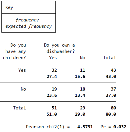   ![](/assets/images/Stata_Chisquare_output.png){:class="img-fluid w-60 mx-auto"}  

   Note that in this case the expected frequencies are all greater than \\(5\\), but if the fifth assumption was violated you could conduct Fisher's exact test using the following command instead:

tab q3 q16_3, exact expected

5. The table for the chi-square test shows how the actual sample data compares with what would be expected if there was no association between having children and dishwasher ownership. The fact that there is a bit of a difference between the observed and expected values provides evidence of association in the sample, with the nature of the association being that people with children are more likely to own a dishwasher.   

   To find out whether the association is significant, we need to refer to \\(p\\) value below the table. Since \\(p < .05\\) (in fact \\(p = .032\\)) we can reject the null hypothesis and conclude that there is a statistically significant association between having children and owning a dishwasher.   
 
   For more information on how to interpret these results see the [_Introduction to statistics_](https://uniskills.library.curtin.edu.au/numeracy/statistics/inferential#chi-square-test) module. 

<h3 id="digital-stata-assessing-relationships-testing-for-linear-correlation">Testing for linear correlation</h3>

A question you may wish to ask of the wider population is: _Is there a statistically significant linear correlation between summer daily energy consumption and winter daily energy consumption?_   

This question can be answered by following the [recommended steps](#digital-stata-inferential-hypothesis-testing), as follows:   

1. The appropriate hypotheses for this question are:  
\\(\textrm{H}\_\textrm{0}\\): There is no significant linear correlation between summer and winter daily energy consumption  
\\(\textrm{H}\_\textrm{A}\\): There is significant linear correlation between summer and winter daily energy consumption  

2. The appropriate test to use is Pearson's correlation coefficient, as we are testing for linear correlation between two variables (summer daily energy consumption and winter daily energy consumption). 

3. The assumptions for Pearson's correlation coefficient are as follows:   
* **Assumption 1:** The sample is a random sample that is representative of the population.   
* **Assumption 2:** The observations are independent, meaning that measurements for one subject have no bearing on any other subject's measurements.   
* **Assumption 3:** The variables are both continuous.   
* **Assumption 4:** Both variables are normally distributed, or the sample size is large enough to ensure normality of the sampling distribution.   
* **Assumption 5:** There is a linear relationship between the variables, as observed in the scatter plot (this is not strictly an assumption as Pearson's correlation coefficient is still valid without it, but if you already know the relationship is not linear further interpretation is not necessary).   
* **Assumption 6:** There is a homoscedastic relationship between the variables (that is, variability in one variable is similar across all values of the other variable), as observed in the scatter plot (dots should be similar distance from line of best fit all the way along). 

   While the first three assumptions should be met during the design and data collection phases, the fourth, fifth and sixth assumptions should be checked at this stage (for instructions on checking the normality assumption in Stata, see the [The normal distribution](https://uniskills.library.curtin.edu.au/digital/spss/normal-distribution) page of this module).   

   If the normality assumption is not met you can try transforming the data or using Spearman's Rho or Kendall's Tau-B instead. You can also use one of these tests if you have ordinal rather than continuous variables, or if there is non-linear correlation.   

   To check for linearity and homoscedasticity, you can create a scatter plot with the independent variable on the \\(x\\)-axis and the dependent variable on the \\(y\\)-axis (for this example these are interchangeable; we will put summer consumption on the \\(x\\)-axis). For instructions on creating a scatterplot in Stata, see the [Graphs](#digital-stata-graphs) page of this module.   

   The scatterplot, with the line of best fit included, should look as follows. This shows that the relationship is approximately linear as the points lie close to the line of best fit. It also shows that the relationship is homoscedastic, as the points are a similar distance from the line of best fit all the way along (they don't create a 'funnel' shape in either direction). Hence the fifth and sixth assumptions have been met.   

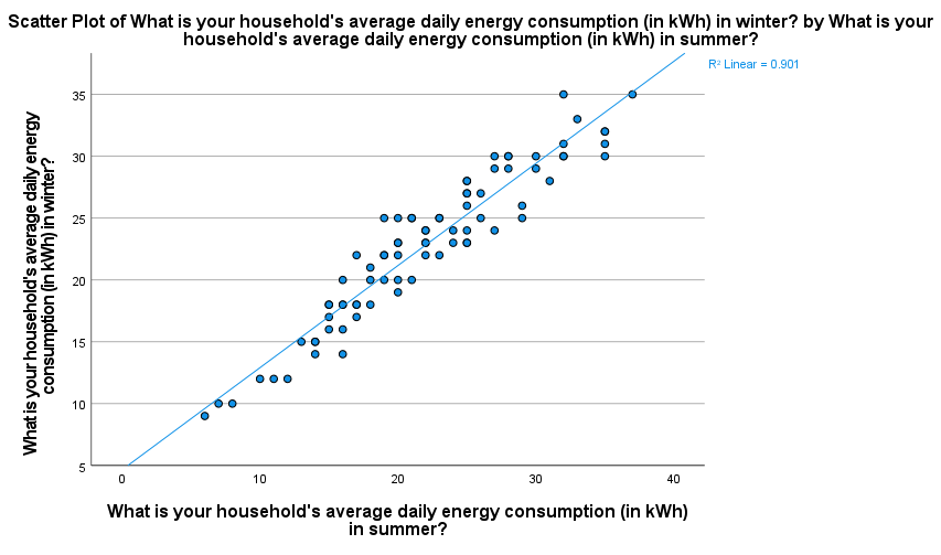   ![](/assets/images/Pearsons_correlation_scatterplot.png){:class="img-fluid w-75 mx-auto"}  

4. If the assumptions are met, you can assess Pearson's correlation coefficient in Stata by running the following command:

pwcorr q6 q7, sig ```

The output should look like this:

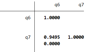
The results of the test of correlation, with correlation coefficient .949 and p value .0000

This table shows that Pearson’s correlation coefficient is \(.949\), indicating a strong positive linear correlation between summer and winter energy consumption (for more information on how to interpret this see the Descriptive statistics page of this module

To test whether this linear correlation is statistically significant requires the \(p\) value (listed directly below the correlation coefficient). Since \(p < .05\) (in fact \(p < .001\)) we can reject the null hypothesis and conclude that there is a statistically significant linear correlation between summer energy consumption and winter energy consumption.

Pearson’s correlation coefficient and its square (the coefficient of variation) are also measures of effect size, which can be used to test for practical significance. The correlation coefficient of \(.949\) indicates a large effect, and the coefficient of variation of \(90.06\%\) indicates that \(90.06\%\) of variation in winter energy consumption can be explained by variation in summer energy consumption.

For more information on how to interpret these results see the Introduction to statistics module. <h2 id="digital-stata-feedback">Feedback</h2>

If you would like to provide feedback on this module please do so by answering some or all of the questions in the form below. Alternatively for any questions about the module please contact Library-UniSkills@curtin.edu.au

We review this feedback regularly, and take your suggestions on board to improve the module. Thank you for your feedback!

Explore more here

About UniSkills

UniSkills was created and is maintained by Curtin University Library. To report issues with UniSkills contact Library Help.

Twemoji icons by Twitter, Inc and other contributors, licensed under a CC-BY 4.0 licence.

Except where otherwise noted, UniSkills content in all it’s forms (website, PDFs etc) are licensed under a Creative Commons Attribution ShareAlike 4.0 International Licence. We ask that you attribute any use of the content as created by Curtin University Library with a link to the Library website.

This license does not extend to other Curtin University and Curtin University Library webpages, or to Curtin branding and trademarks. Curtin University’s copyright information is available on the Curtin website.

age	gender	children	summer_consumption	winter_consumption	household_size	consumption_reduction
21	1	2	17	18	2	4
35	1	1	26	22	4	5
29	2	1	25	28	5	3
46	3	1	19	20	3	4
32	2	2	12	13	1	2
25	2	2	16	18	2	4
41	2	1	26	27	6	2
	2	2	15	16	2	3
26	1	2	32	29	5	5
48	2	1	40	33	7	5

age	gender	children	summer_consumption	winter_consumption	household_size	consumption_reduction
21	1	2	17	18	2	4
35	1	1	26	22	4	5
29	2	1	25	28	5	3
46	3	1	19	20	3	4
32	2	2	12	13	1	2
25	2	2	16	18	2	4
41	2	1	26	27	6	2
	2	2	15	16	2	3
26	1	2	32	29	5	5
48	2	1	40	33	7	5

age	gender	children	summer_consumption	winter_consumption	household_size	consumption_reduction
21	1	2	17	18	2	4
35	1	1	26	22	4	5
29	2	1	25	28	5	3
46	3	1	19	20	3	4
32	2	2	12	13	1	2
25	2	2	16	18	2	4
41	2	1	26	27	6	2
	2	2	15	16	2	3
26	1	2	32	29	5	5
48	2	1	40	33	7	5